Group 1
Faraday waves and pattern formation
Group members: J. Orphee, P. Cardenas-Lizana, M. Lane, E. Grossman
Main presentation, Non-newtonian presentation. Papers: Paul, Juan
Faraday waves are formed when a fluid is vertically vibrated above a critical amplitude / frequency. Faraday waves are a model pattern forming system and a hallmark of nonlinear dynamics. Here we investigate the onset of pattern formation in a vibrated fluid for a variety of experimental conditions.
Introduction
- Eponymously discovered by Faraday[1], Faraday Waves are standing waves on a fluid caused by vertical oscillatory motion. At given frequencies, these standing waves (vibrating at held the driving frequency) give surface patterns of n dimensional rotational symmetry; mainly square, hexagonal, and 8-fold quasi-static patterns. The wavelength of the standing waves are a function of viscosity, surface tension and density. Hence, understanding the relationship between these variables and the wavelength, will allow oscillation frequencies to be selected that produce standing waves of order n [2]:
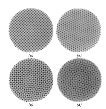

a) n=2 (square symmetry) b) n=3 (hexagonal symmetry) c) n=4 (8-fold quasiperiodic) d) n=5 (10-fold quasiperiodic)
The principle in this experiment is to vibrate a container with liquid vertically at a fixed frequency and amplitude. These waves consist of a standing wave pattern that occurs in a free fluid surface under excitation. At low vibration amplitudes, the liquid moves as a solid body, but at high vibration amplitudes, surface waves start to form. For instance, When a layer of fluid is oscillated up and down with a sufficiently large amplitude, patterns form on the surface, a phenomenon first observed by Michael Faraday in 1831. The standing waves form a pattern on the surface because the amplitude of the excitation exceeds a critical value. The excitation number is defined as $(A-Ac)/Ac$, where the vibration amplitude is denoted by $A$, the onset amplitude for the waves is denoted by $Ac$. This excitation number will define the characteristic of the pattern formation.
A collection of different wave modes compete and which pattern wins depends on the excitation number, the frequency, and the liquid viscosity. It is worth noting that all the modes have the same wave length, and that the wave length is independent of the vibration amplitude. In addition, the patterns observed are approximately independent of the boundary conditions for large enough containers; however if the container is small, the shape of the boundary will interfere and may destroy the pattern formation. The patterns range from squares, hexagons, triangular, and 8-fold quasi-periodic depending on the excitation frequency fluid properties (viscosity, surface tension, and density) Even though this phenomenon has been studied since its discovery by Faraday, a full understanding of the subject has not yet emerged.
Background Theory
The formation of Faraday waves has been studied in several physical context, including convective fluids, nematic liquid crystals, nonlinear optics, biology, and, recently, in Bose-Einstein condensates; where the mechanisms of pattern selection was investigated using the tools of symmetry and bifurcation theory. Faraday waves in Non-Newtonian fluid was also recently studied. It was found that it is possible for holes to be created inside fluids such as cornstarch when undergoing vertical oscillation. Forming at a critical driving shaker acceleration and frequency, these holes are unusual in that their motion is not directly dependent on the Faraday waves, because the holes form far away from each other in the medium and tend to merge if they get to close to each other. Zhang and Vi\~nals have derived and equation that describe Faraday-wave amplitudes in the weakly damped and infinite depth limit. These equation has been tested in the weakly viscous and large depth limit and it provides a good agreement between this theory and experiments under these conditions. This theory predicts that the preferred patterns are the ones in which the Lyaupunov functional is minimized; which predicts for most excitation frequencies a square pattern for low viscous fluids. But for a narrow frequency band, hexagons and other quasi-periodic patterns are predicted. The experimental observation are: at high viscous dissipation, the observed wave pattern above threshold consists of parallel stripes; at lower dissipation, patterns of square symmetry are observed in the capillary regime of large frequencies. At low frequencies, higher symmetry patterns have been observed like hexagonal, and eight- and ten-fold quasi-periodic patterns. However, many of the experiments use shallow viscous layers of fluid to counteract the presence of high frequency weakly damped modes that can make patterns hard to observe. (A map of patterns vs. frequency is know. Current research aims at the study of this nonlinear pattern formation at a finite distance from threshold. It is now known that the evolution of the wave pattern near onset is variational, and its parameter space behavior is small in most fluids and vanishes with the viscous damping parameter. Non-variational corrections are anticipated to be large near onset, and play a important role in Faraday-wave instabilities and on the transition to spatio temporal chaos.
Fundamental Equation Farday Instability
- <math>\nabla\cdot\mathbf{v} = 0</math>
- <math>
\frac{\partial \vec{v}}{\partial t}+\vec{v}\cdot\nabla\vec{v}= -\nabla \rho + \frac{1}{\mathrm{Re}} \nabla\cdot \left(\nabla\vec{v} + \nabla\vec{v}^T \right)+ \frac{1}{Fr}F(cos(2\pi t)-1)\mathbf{j}</math>

Previous Experiments
Binks and van de Water [2] choose to examine the stability of faraday waves as a function of excitation frequency. The wavelength of each mode can be determined from the inviscid deep fluid dispersion relation: ![]() where:
where:
![]() (g is acceleration due to gravity, k is the wave number, and 2w is the excitation frequency)
(g is acceleration due to gravity, k is the wave number, and 2w is the excitation frequency)
![]() (alpha is the surface tension, and rho is the density)
(alpha is the surface tension, and rho is the density)
Furthermore, the theory of this experiment is only valid for gamma << 1 where gamma is
![]() , the inverse Reynolds number.
, the inverse Reynolds number.
With these values, Binks and Water varied the amplitude of the oscillations for different frequencies and plotted the stable points on a phase diagram. In between each stable standing wave was a mixture of both waveforms. These transitionary states were shown to be bicritical points. Peilong and Vinals [4] were able to select stable points as a function of driving frequency and viscosity and plot them in a graph as shown:

Non-Newtonian Fluid Experiments
Non-Newtonian fluids have the property that its viscosity is not constant as stress is applied to it over time. As the phase diagram below shows the higher viscosity, this means that the critical amplitude and frequency required for Faraday waves is higher and up to a point the number of possible Faraday waves will decrease or stop all together above certain of frequencies and amplitude. It is even possible for holes to be created inside fluids such as cornstarch when undergoing vertical oscillation (Goldman [7]). Forming at a critical driving shaker acceleration and frequency, these holes are unusual in that their motion is not directly dependent on the Faraday waves, because the holes form far away from each other in the medium and tend to merge if they get to close to each other. In fact the radius R(t) of a hole is depends on acceleration a, frequency f, and the resonant frequency of the material f0 by the formula:
- <math>
\begin{aligned} R(t) & = K * F(t+\varphi ) \\ F(t) & = Driving Function \\ \tan (\varphi ) & = \frac{\alpha }{1-\frac{f^2}{f_0^2}}\\ \end{aligned} </math> Instead Dr. Goldman and other’s found that it was the stability of these holes to last and remain open is dependent on the magnitude of the maximum shear thickening gamma, which is in turn affected by the viscosity eta and other proprieties of the liquid in question. In general the formula for shear thickening is:
- <math>
\begin{aligned} \eta & =\frac{2 \tau}{\pi \gamma ^{n-1} R(t)^3} & For Non-Newtonian \\ \eta & =\frac{2 \tau}{\pi \gamma R(t)^3} & For Newtonian \end{aligned} </math>
Experimental Setup
This experiment is designed to reproduce the results of Binks and W. van de Water [2] and contrast the results with Zhang and Vi\~nals [3] prediction of the amplitudes of the standing waves. We expect a fair agreement between our experiment and the theory. In addition, our experimental study will move a step further and not only investigate the theory for different fluids, including a non-Newtonian fluid, but for different oscillatory patterns (square, sinusoidal,and triangle) and the importance of the boundary condition for relatively small container. To begin, we will build a basic experimental setup in Dr Goldman's lab using an open container that will be subjected to vertical sinusoidal oscillations, which periodically modulate the effective gravity and capture the amplitude by using a high speed CCD camera. The camera will be placed above the container to take snapshots of the standing waves and the frames per second of the snapshots must be greater than the oscillation period of the standing waves. By using the sinusoidal oscillator, we will also construct our trial waves, which will have the form of square and triangular.
We will calibrate our system by measuring the driving amplitude A that exceeds the critical threshold Ac and cause an standing-wave instability; this occurs with temporal frequency ω that is around one half of the driving frequency as predicted by Faraday. After we have estimates of acceleration at which a pattern first appears, we will be able to observe how these patterns change as the driven amplitude is slowly increased. The characteristic spatial wavelength of the standing-wave pattern can be estimated by the dispersion relation ω(k) of the fluid and the amplitude of the waves can be measured by a laser.
After the building process, we will first reproduce classical results on pattern formation of water and oil to validate our experimental setup. Since the patterns form by water and oil are well documented, we will observe surface standing waves in water and oil with different driven frequencies and amplitudes to verify that our setup is working properly. Experiments will begin with small depth h=3 mm and increase the depth to about 1.5-2 cm. Then we will begin increasing slowly and carefully the driving force amplitude and stop increasing the amplitude when the resonance is strong enough and begin to increase frequency. This part must be done very slowly as every new pattern cannot become stable very fast. Second we will compare patterns obtained and amplitudes with classical results as a function of excitation frequency, for at least two different working fluids, and one being Non-Newtonian; specifically we will study the amplitudes and patterns with theory as a function of driving frequency. By using the Non-Newtonian fluid, we will test if the theory is consistent across different fluids. Third we will also discuss the effects on patterns for different excitation wave forms like sine, square, triangular. Finally, we will study the boundary conditions of the wave-amplitude formation. For this propose, we will use different container shape like cylinder, and box.
All the experiments are performed in the following manner; the frequency is fixed and the amplitude is varied going from 0 to beyond its critical value (Ramp-up) and returning to 0 (Ramp-down). The critical value is where the first Faraday Instability appears. We work with Water, Oil, and a Non-Newtonian fluid with different container shape. Different excitation signal, Sine, Triangular, Square are used. The range of frequencies are between 30Hz to 110 Hz.
Parts List
- Circular Cylinder
- High Speed CCD Camera
- 2 fluids with different viscosities (oils)
- A non newtonian fluid (cornstarch)
- An electromagnetic exciter (or any device that can oscillate vertically)
Procedure

- Reproduce the experiments of Binks and Van de Water
- Fill a 440 mm diameter circular container with 20 mm height of experimental fluid
- Attach a 2 cm thick plate on the bottom of the container and a hollow conical structure attached to an electromagnetic exciter below that.
- Place piezo-electric accelerometers on the cone (one on bottom, two on top) to measure the acceleration cone. This allows control of the oscillation frequency.
- A high speed CCD camera is placed above the container to take snapshots of the standing waves. It is required that the frames per second of the snapshots are greater than the oscillation period of the standing waves.
- The amplitude of the oscillations are controlled by the electromagnetic exciter and increased in small steps (about 1%) where each wave is held for 2000 seconds first before taking 1000 s of images of the waves.
- Measurements of the amplitude of the waves are taken by a laser
- Compare the amplitudes and patterns with theory as a function of driving frequency
- Repeat experiment with another fluid, and a non newtonian fluid and checking if theory is consistent across different fluids.
- Observe the effects of changing the wave form on the standing waves
- Sinusoidal Waves
- Square Waves
- Triangle Waves
The shaker is expensive and delicate. we must set the amplifier gains to minimum before turning on the system, gradually turning up the gain knob during use. The input frequency should never exceed 130 Hz. The range of interest for Faraday waves for our system is $10Hz \leq f \leq 100Hz$. If you see and hear the typical features of beats instead of a harmonic mode of vibration, immediately set the amplitude to zero with following adjustment of the driven frequency, just to shift the mode of vibration away from the dangerous state.
Visualization Of Faraday Waves
The following videos were taken when we were performing the Faraday wave experiment.
<videoflash>YCP_5h8KF6U</videoflash>
<videoflash>r3p_sMSP8s8</videoflash>
<videoflash>6TzrxxRYM2o</videoflash>
<videoflash>tgo9mOgwDPc</videoflash>
Results & Discussion
NonNewtonian Results
The intial plan for the Non-Newtonian part of our experiment was simply to measure and observe the similarities between the Non-Newtonian Faraday Waves and the Driving Signal Wave as well as observe the unique phenomena of holes and fingers that occur when on introduces a pertibation (see the video below). We decided to compare the bifurcation diagrams of Cornstarch to Water.
<videoflash>M_qXzyaIKI4</videoflash>
 Early on we ran into an issue that there were a range of different values for the recipe and chemical properties of Non-Newtonian cornstarch mixture. Some researchers prefered to use Cornstarch with a oil while others simply used cornstarch and water. In fact, water mixed with cornstarch is a special Non-Newtonian called oobleck, coined by Dr. Suess. has an important role in teaching the physical chemstry for elementary school students. In order to figure out the ideal concintration we looked at how the upward onset of the Faraday instability bifurcation vs. concintration. As the figure above shows, the bifurcation asymptotically increases soon after a reciepe ratio of 2 parts cornstarch to 1 part water. For the rest of the experiment, we used a concintration of 2.5 : 1 since it seem to a fai upward bound.
Conclusion
As the first video shows, we qualitatively observed holes and rising columns the unique pertibative properities. Above a critical acceleration, these holes remain persistant due to the thickening of the fluid. In fact the shearing pressure and strain of the pertibation causes water to dissolve out of the cornstarch solvent. As soon as the water is displaced, the free cornstarch molecules reform solid ionic bonds which then give the liquid it shear thickening properties.sd
Below is a video of the experiment we ran to measure the bifurcation for cornstarch.
<videoflash>IVxmY0CDF5g</videoflash>
In the video is abundantly clear that some cornstarch suspension is resists the driving amplitude and does not. In fact in some cases it seem like the solid-like layer of cornstarch was under the oscillating one. One theory for this inhomogenous boundary suggests that the inhomogenity is a result of the aging effects and packing of cornstarch as it is driven. Looking at the bifurcation diagrams we also see a jitter effect (*see N.J. Balmforth et al.) that causes an error in the parameter h/K that controls the vertical y(x=0) intial height of the bifurcation diagram. Please note that curve in the plot below is simply the Taylor-Coulette Landau Equation provided in Strogatz page 88, Problem 3.6.6.

Newtonian And Non-Newtonian Fluid
Water is excited at 30Hz, and the forcing acceleration (the base shaking amplitude) is increased continuously from zero up to a maximum value, referred as the "ramp-up" in Figure below. As the forcing acceleration increases, a critical acceleration is reached, (critical acceleration "up"), at which the Faraday waves start to form. At this critical acceleration "up" the wave amplitude exhibits a rapid increase with increasing forcing acceleration. If the forcing acceleration is increased further, the amplitude of the Faraday wave keeps increasing until the pattern becomes unstable. At this point, the input acceleration is decreased, "ramp-down", and the amplitude decreases back to zero. However, the "ramp-up" path and the "ramp-down" path are different, showing a hysteresis behaviour, as discussed in theory drction. This hysteresis is consistent with a subcritical bifurcation, as depicted by the curve fit in Figure below.

Normalized amplitude (amplitude/maximum amplitude) for water excited at 30Hz, for "ramp-up" path and "ramp-down" path, and corresponding bifurcation curve fit of the type: $0 = \epsilon -gx^2 -kx^4$.
The hysteresis and amplitude saturation arise due to a detuning effect of the natural frequency of the Faraday wave with respect to the excitation frequency. This detuning is caused by the fact that the natural frequency of the Faraday wave is a nonlinear function of its amplitude. Therefore, the natural frequency will be different for the case in which the amplitude is zero, acceleration increasing "ramp-up" path from rest, than when the amplitude is non zero, corresponding to a decrease in acceleration "ramp-down" path. The different natural frequencies means that the wave will be close or far from being in resonance with the forcing frequency. As the critical acceleration up is reached, the wave frequency response is in close proximity to being resonant; and thus, very unstable, with any perturbation causing the wave to form and increase in amplitude rapidly. However, as the amplitude grows, the natural frequency of the wave shifts away from resonance and the amplitude diminishes its growth rate, it saturates. This saturation is model by including a fifth order term in the amplitude equation, which balances the growth of the cubic term. Similarly, the subcritical behaviour can be observed for a range of excitation frequencies 30-110Hz, as shown in Figure below, but the actual bifurcation shape will change for each frequency. For higher frequencies, the amplitudes and wavelengths become smaller. And for the highest frequency tested, 110Hz, the amplitudes are much smaller and the pattern becomes unstable. The bifurcations have been fitted with amplitude eqn., and the fit coefficients are shown in Table below. As predicted by the theory for a subcritical bifurcation, $g < 0$ and $k > 0$. Where k is the coefficient of the fifth order term, which is stabilizing and responsible for modelling amplitude saturation. And $g < 0$, corresponds to the cubic, de-stabilizing, term. Also, in order to explore the consistency of the particular bifurcation for each frequency, the experiment is repeated 5 times for each frequency, Figure below. The general bifurcation shape is repeated, and thus there is a unique response of the fluid for a given excitation frequency. Also, there are approximate bounds for the critical accelerations "up" and "down".


Similarly, for the non-Newtonian fluid, the bifurcation behaviour is examined for a range of frequencies and compared with water, Figure above. For the non-Newtonian fluid, the critical accelerations required are much higher due to a higher viscous dissipation, higher viscosity value as compared with water. Also, the shape of the bifurcation and its hysteresis are quite different as compared to water. For non-Newtonian fluids, the pattern may continue to exist for higher forcing accelerations, but its amplitude response shows a strong saturation, remaining almost flat, or in some cases even decreasing with increasing forcing acceleration.
Since for a subcritical bifurcation, the system becomes unstable as the acceleration gets closer to the critical "acceleration up," a perturbation experiment is conducted, Figure below. In this experiment, the container is physically tapped continuously as the acceleration is increased. As expected, the Faraday waves form before the critical acceleration up of the undisturbed system is reached. Also, as the acceleration is ramped down, the amplitude for the disturbed system reaches a critical "acceleration down" that is lower than the undisturbed system. This latter effect is surprising and may be due to the introduction of noise in the system which may widen the forcing frequency bandwidth, and increases the chances for the natural frequency of the Faraday wave to be closer to resonance with the forcing frequency, thus attenuating the amplitude decay with decreasing acceleration. This supposition is further reinforced by the next test, which compares a triangular wave input, with the base case, a sinusoidal input, Figure below. The triangular wave in spectral space is composed on infinite number of wave numbers, and thus again this widens the forcing frequency spectrum; thus, increasing the chances that the natural frequency of the Faraday wave is tuned to some of the forcing wave numbers, and the amplitude decreases at a lower critical acceleration down. This same reasoning applies for the increasing amplitude case, which explains why the critical acceleration up happens before than for the sinusoidal input.

Furthermore, square wave inputs have been explored, but resulted in a wave pattern containing multiple wave numbers, Figure above, and amplitude measurements become ambiguous.
The critical acceleration up and down as a function of frequency are shown for water and the cornstarch mixture in Figure below. As explained in the theory section, the critical acceleration increases with increasing frequency and viscosity due to the increase in dissipation at the boundaries of the container. And since in this experiment the viscosity of the non-Newtonian fluid is much higher than water, much higher critical accelerations are required to form a pattern.

The wavelength as a function of frequency for water and cornstarch mixture is also explored, Figure below, and compared with the theoretical approximation of $\lambda \sim {1/f}$ for shallow fluid depth. The results are in overall agreement with the theory, curve fits shown, for Newtonian and Non-Newtonian fluid.

As mentioned, there is a maximum, saturated, amplitude for each forcing frequency, as shown in Figure below. While to the author there is no explicit theory that predicts the behaviour of the saturated amplitude versus forcing frequency, it seems that for larger frequencies $A_{max} \sim 1/f$. However, at 30Hz the maximum amplitude seems not to fit this approximation well, being surprisingly, about twice the amplitude of the 40Hz case.

Finally, the bifurcation departure of our experiment are compared in a qualitative manner with results from Wernet et al., since experimental set-up and working fluids are different. Wernet et al. explored an amplitude departure for a working fluid with ~10 times the viscosity of water and the container used was carefully designed to avoid meniscus induced waves, "soft-beach" boundaries. Wernet et al. also tried to model the bifurcation without a fifth order saturating term; however, his work does not indicate whether this set-up induces a hysteresis behaviour. For the 60Hz, Wernet et al. shows a rapid increase of amplitude that resembles the sharp departure at "ramp-up" exhibited by water, Figure below. And at 80Hz, the results from Weret et al. show a slower departure from zero than water, but the cubic term amplitude departure (represented by the square root curve fit) seems not to agree well the amplitude saturation, which appears better captured with a fifth order term, shown by the subcritical bifurcation curve fit,


Other Captured Phenomena (Videos)
We also observe the following Phenomena.
<videoflash>Thp8GKIL-iM</videoflash>
<videoflash>LPtQdXyCx9g</videoflash>
This Lab
Other Labs
Faraday Waves on Cornflour
Faraday Waves set to music
Conclutions
In summary, the main goal of this project is to study the nonlinear behavior of the pattern formation on the Faraday experiment. The problem is formulated for general contrasting the theory with experimental results. Although, we focus on a few particular cases, where only few parameters are measured and controlled, our experimental design, at the same time, can provide new insights since there is still a lack of full understanding of this phenomenon. For the chosen working fluids, water and mixture of water with cornstarch, and this experimental setup, Sub-critical behavior of Faraday waves is observed. Different input signals generate different wave forms, with different critical accelerations, and amplitudes. A confirmation of wavelength $\approx1/freq$ is observed for Newtonian and non-Newtonian fluids. Maximum amplitudes are in overall agreement with experimental results from Wernet et al. Finally in our experiments potential new findings are found. The critical accelerations seem to vary linearly with frequency for both Newtonian and non-Newtonian fluids and maximum amplitudes tend to scale with $\approx1/freq$ for increasing frequency. To the best to our knowledge, there is no theory that predicts this behavior.
Group Members
- Juan Orphee
- Paul Cardenas-Lizana
- Michael Lane
- Elan Grossman
Sources
- [1] M. Faraday, Philos. Trans. R. Soc. London 121, 319 (1831)
- [2] D. Binks and W. van de Water, Phy. Rev. Lett. 78, 4043 (1997) <http://alexandria.tue.nl/openaccess/Metis132530.pdf>
- [3] W. Zhang and J. Viñals, Phys. Rev. E 53, R4286 (1996)
- [4] Peilong Chen and J. Vinals, Phys. Rev. Lett, 79, 2670 (1997) <http://homepages.spa.umn.edu/~vinals/mss/peilong1.pdf>
- [5] J. Bechhoefer and B. Johnson, Am. J. Phys, 64, 12 (1996). <http://arxiv.org/pdf/patt-sol/9605002v1>
- [6] A. Kudrolli and J.P. Gollub, Physica D 97, 133 (1996)
- [7] Florian S. Merkt, Robert D. Deegan, Daniel I. Goldman, Erin C. Rericha and Harry L. Swinney, PRL 92, 184501 (2004) <https://www.physics.gatech.edu/files/u347/public/prl84501.pdf>