Group 3
Group members: Nitin Arora, Phillip Gray, Chris Rodesney, Jacob Yunis

The appropriately-named bouncing inelastic ball experiment is composed of a perfectly inelastic ball bouncing on an oscillating plate. It is a simple yet elegant system that exhibits striking nonlinear behavior. On this page, we construct a computational model using various forcing waveforms for the plate, and generate associated bifurcation diagrams. We also explore experimentally the case of a harmonically forced plate.
Theory
The system of a ball bouncing completely inelastically on a vibrated platform has been the subject of numerous studies <ref>A. Mehta and J. M. Luck, Physical Review Letters 65, 393 (1990)</ref> <ref>T. Gilet, N. Vandewalle, and S. Dorbolo, Physical Review E 79, 055201(R) (2009)</ref>, and the case of a simple harmonically vibrated plate was completely resolved by Gilet et al. The primary means for analyzing the motion is measuring the time of flight between successive impacts of the ball with an n-cycle corresponding to the ball having n unique flight times before repeating. For small forcing, Gilet et al found an alternating series of one and two cycles with a small region containing an infinity of bifurcations around control parameter $\Gamma \simeq 7.253378$.
We investigate the case of a plate vibrated according to a superposition of two sine waves with a frequency ratio $c$:
<math> \begin{equation} x_p(t) = A[\sin(\omega t) + \sin(c \omega t)] \end{equation} </math>
The ball can take off from the plate when the acceleration of the plate is less than negative g, the acceleration due to gravity:
<math> \begin{align} \ddot{x}_p(t) = -A[\omega^2\sin(\omega t) + c^2 \omega^2\sin(c \omega t)] &\leq -g \notag\\ \frac{A\omega^2}{g} [\sin(\omega t) + c^2 \sin(c \omega t)] &\geq 1 \end{align} </math>
In this way, the motion of the ball from initial takeoff at <math>t_0</math> is:
<math> \begin{align} x_b(t) = &x_p(t_0) - x_p(t) + \dot{x}_p(t_0)(t-t_0) - 1/2 g(t-t_0)^2 \notag\\ x_b(t) = &A[\sin(\omega t_0)+ \sin(c \omega t_0) - \sin(\omega t) - \sin(c \omega t)] + A[\omega \cos(\omega t_0) + c \omega \cos(c \omega t_0)](t-t_0) - 1/2 g(t-t_0)^2 \notag \end{align} </math>
<math> \Gamma, \varphi, \chi</math> regime
The above functions can be made dimensionless via the introduction of a characteristic time <math>1/\omega</math> and a characteristic length <math>g/\omega^2</math>. We can thus define a phase <math>\varphi = \omega t</math>, a reduced acceleration and one of our control parameters <math>\Gamma = A\omega^2/g</math>, and a generalized position <math>\chi = A\omega^2/g</math>. The other control parameter is the ratio of the frequencies <math>c</math>.
The forcing of the plate is now given by:
<math> \begin{equation} \chi_p(\varphi) = \Gamma(\sin(\varphi) + \sin(c \varphi)) \end{equation} </math>
The position of the ball relative to the plate is
<math> \begin{align} \chi_b(\varphi) = &\Gamma[\sin(\varphi_0)+ \sin(c \varphi_0) - \sin(\varphi) - \sin(c \varphi)] + \dots \\ &\Gamma[\cos(\varphi_0) + c\cos(c \varphi_0)](\varphi - \varphi_0) - 1/2(\varphi-\varphi_0)^2. \notag \end{align} </math>
and the ball takes off when
<math> \begin{equation} \Gamma [\sin(\varphi) + c^2 \sin(c \varphi)] \geq 1 \end{equation} </math>
Period Doubling and Chaos
The flight time is defined as <math>T = \varphi_i - \varphi_0</math>, and can be found by solving the following equation numerically:
<math> \begin{align} F \equiv &\Gamma [\sin(\varphi_0)(1-\sin T) + \sin(c\varphi_0)(1-\sin cT) - \cos T \cos(\varphi_0) - \cos(cT)\cos(c\varphi_0)] - \dots \\
&\Gamma[\cos(\varphi_0) + c\cos(c\varphi_0)]T - 1/2 T^2 = 0
\end{align} </math>
The ball is able to land in two distinct regions. There is a 'bouncing' region, where the acceleration of the plate is such that the ball will immediately take off again, with an initial velocity equal to the instantaneous velocity of the plate at the time of impact. The other region is the 'sticking' region, where the ball is not able take off, and instead rests on the plate until the plate's acceleration is such that is can take off again. This region is a sort of resetting region, as the ball immediately forgets any history it had prior to landing. The sticking region will mark the boundary between periodic cycles.
By varying the control parameter <math>\Gamma</math> we construct bifurcation diagrams for the cases <math>c=1, c=2</math> and <math>c=3</math>.
Bifurcation Diagrams
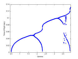
<math>c=1</math>
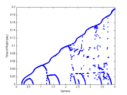
<math>c=2</math>
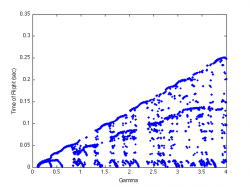
<math>c=3</math>


Experiment
The experimental setup involves a horizontal shaking platform driven vertically according to the forcing function inputted by an oscilloscope or computer. A small, inelastic ball is placed on the plate and it's motion is recorded by a high speed camera. The camera data is then transferred into position data for both the ball and the plate to be compared with the predictions made by our computational model. Below is a list of required components.
Parts list
- oscilloscope or computer capable of outputting different forcing functions
- shaker plate
- completely inelastic hacky-sack type ball
- high speed camera with computer interface
- tracking software
Results
To be found.
References
<references />