Inverted pendulum-2010: Difference between revisions
JeffAguilar (talk | contribs) No edit summary |
JeffAguilar (talk | contribs) No edit summary |
||
| Line 34: | Line 34: | ||
to the level necessary for the shaker. Acceleration data was also sent to an oscilloscope, from which the peak acceleration could be monitored independently of the controller. | to the level necessary for the shaker. Acceleration data was also sent to an oscilloscope, from which the peak acceleration could be monitored independently of the controller. | ||
[[File:ipsetup.jpg | center | | [[File:ipsetup.jpg | center | 500px]] | ||
A high speed camera was mounted directly in front of the pendulum, and took photos at up to 200 frames per second (fps). The higher speeds caused erratic frame rates, so the camera was generally operated at 100 fps. The images were sent to a second computer with a Labview tracking program. The program applied a threshold of luminance to identify the spot, and tracked the centroid of the spot within a torus section selected by the user. The program was able to track the relative x and y position of the dot, from which the angle of the pendulum could be extracted. While the pendulum was in the stable inverted position, the vertical displacement of the pendulum equaled the vertical displacement of the shaker table, and so could be used to determine the amplitude of the forcing displacement. To determine the region of stability, we recapitulated our procedure from the numerical trials. We varied the driving frequency from 20Hz to 50Hz, and the eccentricity from 0 to 0.999. At each node, we attempted to increase the acceleration until the inverted pendulum became stable in the upright position. For those nodes that we could stabilize, we then decreased the acceleration slowly until stability was spontaneously lost. We then returned the pendulum to stability and recorded the acceleration and the displacement of the forcing function. This process had two main sources of noise: it was difficult to fine tune the acceleration to within 1g; at the boundary of stability, it was sometimes subjective whether the pendulum was truly stable. | A high speed camera was mounted directly in front of the pendulum, and took photos at up to 200 frames per second (fps). The higher speeds caused erratic frame rates, so the camera was generally operated at 100 fps. The images were sent to a second computer with a Labview tracking program. The program applied a threshold of luminance to identify the spot, and tracked the centroid of the spot within a torus section selected by the user. The program was able to track the relative x and y position of the dot, from which the angle of the pendulum could be extracted. While the pendulum was in the stable inverted position, the vertical displacement of the pendulum equaled the vertical displacement of the shaker table, and so could be used to determine the amplitude of the forcing displacement. To determine the region of stability, we recapitulated our procedure from the numerical trials. We varied the driving frequency from 20Hz to 50Hz, and the eccentricity from 0 to 0.999. At each node, we attempted to increase the acceleration until the inverted pendulum became stable in the upright position. For those nodes that we could stabilize, we then decreased the acceleration slowly until stability was spontaneously lost. We then returned the pendulum to stability and recorded the acceleration and the displacement of the forcing function. This process had two main sources of noise: it was difficult to fine tune the acceleration to within 1g; at the boundary of stability, it was sometimes subjective whether the pendulum was truly stable. | ||
| Line 40: | Line 40: | ||
== Results == | == Results == | ||
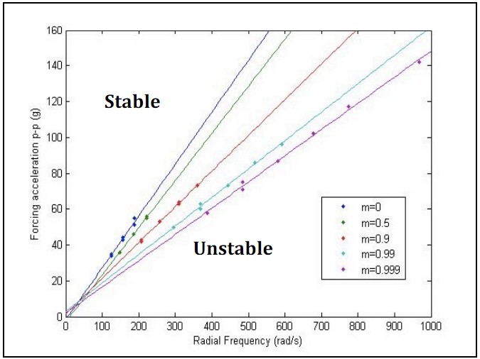
The figure below is a scatter plot of stable points at the stability boundary for each value of m as a function of forcing acceleration (in units of gravitational acceleration - g) and radial frequency (rad/s). Best-fit lines for each value of m is fitted base on the data points. For each value of m, the forcing acceleration required for stability is a linear function of the frequency. Results also show that the lower the value of m, the smaller the region of stability and vice versa. | |||
[[File: | [[File:ipfigure5.jpg | center | 400 ]] | ||
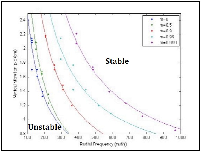
The figure below shows the scatter plot for the same experimental data points for each value of m, but as a function of vertical variation (cm) and radial frequency (rad/s). In this plot, for each value of m, displacement has inverse relationship with frequency. Results also show that the lower the value of m, the smaller the region of stability and vice versa. | |||
[[File:ipfigure6.jpg | center | 400 ]] | |||
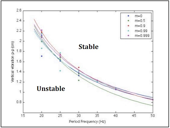
The figure below shows the scatter plot for the same experimental data points for each value of m, but as a function of vertical variation (cm) and period frequency (Hz). Period frequency is equal to radial frequency/2π. In this plot, for each value of m, displacement has an inverse relationship with frequency. However, unlike earlier results, there are no significant differences between the regions of stability for the different values of m. | |||
[[File:ipfigure7.jpg | center | 400 ]] | |||
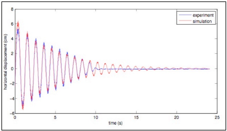
We iteratively adjusted the value of Q in the equation of motion until a good fit is obtained between the simulated displacement and observed displacement (see below). The value of Q is found to be 11 for this system. | |||
[[File:ipfigure8.jpg | center | 400 ]] | |||
The figure below shows the stability diagram for the inverted pendulum as a function of relative amplitude and relative frequency, based on simulation results. For each value of m, displacement has inverse relationship with frequency. Similar to experimental results, there are no significant differences between the regions of stability for the different values of m. Symbols in the diagram represent the actual data points. Results clearly show that there is a constant offset between simulation and experimental results. | |||
[[File:ipfigure9.jpg | center | 400 ]] | |||
== Group Member Bios == | == Group Member Bios == | ||
Latest revision as of 17:47, 23 September 2012
Stabilizing an inverted pendulum
Group members: Yiwei Cheng, Samuel Shapero, M. Robert Hayward
Main presentation. Papers: Yivei, Robert, Samuel
This page is dedicated to the Inverted Pendulum Project. The simulations and laboratory experiments conducted in the inverted perdulum project are part of the requirements of the class: Phys 4267A/6268 Nonlinear Dynamics & Chaos, Spring 2010.
The overarching scientific objective of our research is to provide a coherent picture on stability and bifurcations of an inverted pendulum subjected to forcing that ranges from harmonic to nonharmonic in nature through a combination of numerical studies and laboratory experiments.
Introduction
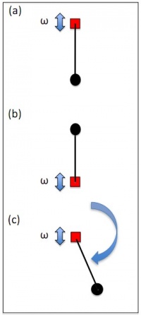
The simple pendulum has only one stable state of equilibrium, which is the vertically down orientation (a). But if the axis undergoes vertical perturbation, three different equilibrium states emerge: (a) stable down, (b) stable up, and (c) Continuous rotation in either direction. The dynamics of an inverted pendulum while subjected to periodic forcing were investigated numerically and experimentally. The following questions were to be answered.
1. What amplitudes and frequencies of periodic forcing allow the inverted pendulum to remain upright? (i.e. what are the regions of stability?) 2. Does the region of stability change when additional harmonics are added to the forcing function? 3. Can our theoretical findings be validated through laboratory experiments?
Modeling
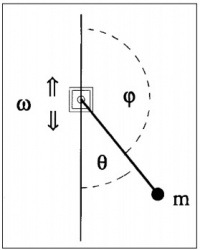
The following equation of motion was employed and integrated with a fourth order Runge Kutta approximation in matlab to compute numerical solutions.
<math>\frac{\delta v}{\delta t}=-\frac{v}{Q \Omega}-\left[\frac{1}{\Omega^{2}}-\epsilon*cn(t,m)\right]*\sin{\theta}</math>
<math>\frac{\delta \theta}{\delta t}=v</math>, <math>Q = \frac{\omega_{0}I}{b}</math>
where $I$ is moment of inertia, $b$ is damping coefficient, $\Omega$ is forcing frequency relative to natural frequency, $\omega_{0}$, and $cn$ is the Jacobi elliptic function used for non-sinusoidal forcing. In order to find the boundary of stability numerically, we swept systematically through values of $\Omega$. For each value of Ω a binary search was used to narrow in on a value of $\epsilon$ lying on the edge of stability. In order to judge stability an initial condition $(\theta, \dot{\theta}) = (1e − 6, −1e − 6)$ was integrated for 1000 periods of the forcing function and checked for divergence.
Methods
In order to verify the accuracy of our Matlab simulations, we set up an inverted pendulum arm on a shaker table with controllable acceleration. The shaker table was attached to a magnetic actuator that converted an electrical signal into mechanical force, similar to a speaker. An ADXL321 accelerometer was mounted to the underside of the shaker, in order to monitor the acceleration for feedback and recording. A signal of 50mV per g of acceleration was sent to a computer with a Labview testbench that controlled the waveform. The software controlled the amplitude of each harmonic component separately, permitting a wide range of waveforms, including Jacobi Elliptics of varying eccentricity. This signal was then broadcast to an VTS-500 high powered amplifier, which boosted the signal to the level necessary for the shaker. Acceleration data was also sent to an oscilloscope, from which the peak acceleration could be monitored independently of the controller.
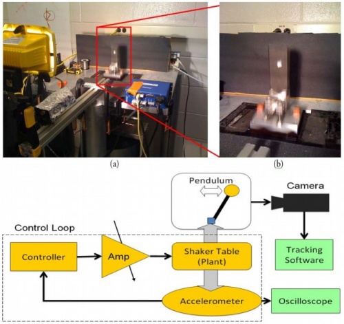
A high speed camera was mounted directly in front of the pendulum, and took photos at up to 200 frames per second (fps). The higher speeds caused erratic frame rates, so the camera was generally operated at 100 fps. The images were sent to a second computer with a Labview tracking program. The program applied a threshold of luminance to identify the spot, and tracked the centroid of the spot within a torus section selected by the user. The program was able to track the relative x and y position of the dot, from which the angle of the pendulum could be extracted. While the pendulum was in the stable inverted position, the vertical displacement of the pendulum equaled the vertical displacement of the shaker table, and so could be used to determine the amplitude of the forcing displacement. To determine the region of stability, we recapitulated our procedure from the numerical trials. We varied the driving frequency from 20Hz to 50Hz, and the eccentricity from 0 to 0.999. At each node, we attempted to increase the acceleration until the inverted pendulum became stable in the upright position. For those nodes that we could stabilize, we then decreased the acceleration slowly until stability was spontaneously lost. We then returned the pendulum to stability and recorded the acceleration and the displacement of the forcing function. This process had two main sources of noise: it was difficult to fine tune the acceleration to within 1g; at the boundary of stability, it was sometimes subjective whether the pendulum was truly stable.
Results
The figure below is a scatter plot of stable points at the stability boundary for each value of m as a function of forcing acceleration (in units of gravitational acceleration - g) and radial frequency (rad/s). Best-fit lines for each value of m is fitted base on the data points. For each value of m, the forcing acceleration required for stability is a linear function of the frequency. Results also show that the lower the value of m, the smaller the region of stability and vice versa.
The figure below shows the scatter plot for the same experimental data points for each value of m, but as a function of vertical variation (cm) and radial frequency (rad/s). In this plot, for each value of m, displacement has inverse relationship with frequency. Results also show that the lower the value of m, the smaller the region of stability and vice versa.
The figure below shows the scatter plot for the same experimental data points for each value of m, but as a function of vertical variation (cm) and period frequency (Hz). Period frequency is equal to radial frequency/2π. In this plot, for each value of m, displacement has an inverse relationship with frequency. However, unlike earlier results, there are no significant differences between the regions of stability for the different values of m.
We iteratively adjusted the value of Q in the equation of motion until a good fit is obtained between the simulated displacement and observed displacement (see below). The value of Q is found to be 11 for this system.
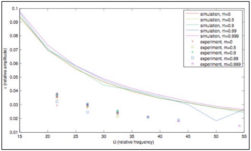
The figure below shows the stability diagram for the inverted pendulum as a function of relative amplitude and relative frequency, based on simulation results. For each value of m, displacement has inverse relationship with frequency. Similar to experimental results, there are no significant differences between the regions of stability for the different values of m. Symbols in the diagram represent the actual data points. Results clearly show that there is a constant offset between simulation and experimental results.
Group Member Bios
Samuel Shapero is a second year PhD student in the Bioengineering Interdisciplinary Program at Georgia Tech. His research focuses on implementing a sparsity extraction algorithm for high dimensional inputs using nonlinear analog circuits. He has a Master’s in Electrical Engineering from Stanford, and has a strong background in analog and digital filter analysis. His research advisor is Dr. Paul Hasler.
Robert Hayward is currently working on PhD in Nuclear and Radiological Engineering (expected Fall 2010). He has strong background in modeling and simulation, numerical analysis and data analysis. He has received his Bachelor’s in Cell and Molecular Biology and Bachelor’s in Mathematics from Tulane. He has received his Master’s in Medical Physics from Georgia Tech.
Yiwei Cheng is a third year PhD student in the School of Civil and Environmental Engineering. Yiwei’s main thesis advisor is Dr Marc Stieglitz and his research focuses on understanding how eco-hydrological processes scale. Specifically, whether there are emergent properties that manifest at scale resulting from small scale non-linearity and feedbacks. His research focus areas are in the Arctic and Everglades Florida, where he conducts field experiments and simulations. Yiwei has received his Bachelor’s and Master’s in Civil Engineering from Georgia Tech.