Group 1 2012: Difference between revisions
Group4 2012 (talk | contribs) No edit summary |
Group4 2012 (talk | contribs) No edit summary |
||
| Line 5: | Line 5: | ||
[[File: Tw_duffing.png | frame | Phase portrait of a duffing oscillator [http://en.wikipedia.org/wiki/File:Tw_duffing.png]]] | [[File: Tw_duffing.png | frame | Phase portrait of a duffing oscillator [http://en.wikipedia.org/wiki/File:Tw_duffing.png]]] | ||
= | <blockquote>We compare a mechanically forced double-well Duffing oscillator with an asymmetric potential to numeric simulations of a symmetric potential system. Analysis is performed with time series data, phase portraits, recurrent Poincare sections, attractor reconstruction from time delay embedding, and Lyapunov exponent estimation from this reconstruction. Our investigation finds that the asymmetric mechanical system can exhibit chaos while for the same forcing parameters symmetric simulation produces limit cycles above or below the chaotic threshold depending on the mechanical potential well used to estimate simulation parameters. | ||
</blockquote> | |||
= Introduction = | |||
The | The forced Duffing oscillator is a seminal system for the study of chaotic dynamics and development of analytical and experimental techniques for nonlinear systems. A common physical interpretation for the double-well case of the Duffing oscillator model considered here is a ferromagnetic beam positioned between two magnets while undergoing lateral forcing, as illustrated in Figure~\ref{fig:beam_illustration}. This mechanical system elucidates several features of the model Duffing oscillator: a potential for the lateral position of the beam created by the two magnets; non-autonomous forcing resulting in motion of the beam, potentially chaotically between the two wells; and mechanical dissipation within the beam and from air resistance against the beam's motion. | ||
Though the Duffing oscillator and the double-well beam system are simple and not of any obvious utility in their own right, they provide a structured model with few, well-defined parameters and clear physical interpretations while still producing chaotic dynamics. This allows intuition into the system's behavior and creates an accessible and familiar setting for experimental design, data analysis, and diagnosis of unexpected results. All these features are valuable both for pedagogical purposes and for the development of new methods and tools for analysis, experimentation, computation, and diagnosis that may be extensible to more complex systems or other scientific or engineering applications. | |||
The Duffing oscillator is | The periodically-forced Duffing oscillator is a system governed by the following nonlinear and nonautonomous second-order ODE (``The Duffing Equation"): <math>\ddot{x}+\delta \dot{x}-\alpha x+\beta x^{3}=f \cos(\omega t)</math> for constants <math>\alpha,\beta,\delta,\omega,f>0</math>. Although it can be viewed as a planar (2 dimensional) system, the nonautonomous periodic term <math>f \cos(\omega t)</math> means that the equation actually determines a smooth vector field on <math>\mathbb{R}^{2}\times \mathbb{S}^{1}</math> (a 3 dimensional space) and hence truly chaotic behavior is possible. | ||
< | To begin to understand this equation, it is simplest to first analyze the case where <math>\delta=f=0</math>. In this case our equation reduces to <math>\ddot{x}-\alpha x+\beta x^{3}=0</math> which is a Newtonian system with potential <math>V(x)= \frac{\beta }{4}x^{4}-\frac{\alpha}{2} x^{2}</math> and the trajectories are curves of constant energy <math>E(x,\dot{x})=\frac{1}{2}\dot{x}^{2}+V(x)</math>. In this case it is easy to see that we have a saddle at the origin and centers at <math>\left(\pm\sqrt{\frac{\alpha}{\beta}},0\right)</math>. Other than the two homoclinic orbits from the origin to itself and the two centers, we have that all other trajectories are in fact closed orbits. | ||
Now when we include the dissipation term (i.e. we let <math>\delta>0</math>), the system is again easy to understand: heuristically, trajectories spiral into what are now stable fixed points at <math>\left(\pm\sqrt{\frac{\alpha}{\beta}},0\right)</math>. We can see that in this case <math>\frac{d}{dt}E = \dot{x}(\ddot{x}+\beta x^{3}-\alpha x)=-\delta\dot{x}^{2}\leq 0</math> so the energy decreases (strictly, when <math>\dot{x}\neq 0</math>) along trajectories of the system. The origin is still a saddle in this case. It can be shown that, except for the stable manifolds of the saddle, all trajectories of this system tend toward one of the stable fixed points. | |||
When we let <math>f>0</math>, the behavior of the system becomes quite complicated. For sufficiently small values of ''f'' we find that we have stable limit cycles near what were stable fixed points for <math>f=0</math>, and almost all trajectories eventually converge to one of the two limit cycles (namely all except for the measure zero stable manifolds of the saddle point at the origin). For very large ''f'', it can be shown there is one globally stable limit cycle attracting all trajectories. For intermediate values of ''f'', however, we have chaotic behavior of trajectories in phase space. This is essentially due to the fact that as we increase ''f'' from 0, we eventually cause the stable and unstable manifolds of the saddle at <math>(0,0)</math> to intersect, and hence to intersect infinitely many times. The presence of infinitely many homoclinic intersection points in (a compact region of) phase space causes the trajectories to have very complex topological structures. These can be seen most clearly via the Poincaré section (sampling the orbit at time intervals of length <math>\frac{2\pi}{\omega}</math>), which displays intricatre fractal ``strange attractors" for these chaotic values of ''f''. | |||
In our experiment, we constructed a mechanical system whose behavior is approximately governed by the above equation. In essence, we used two magnets placed symmetrically about the tip of a strip of shim stock to give us a system behaving like <math>\ddot{x}=-\delta \dot{x}+\alpha x-\beta x^{3}</math>. Here ''x'' denotes the displacement of the tip of the stock, with the vertical beam giving us ''x''=0 and the magnets being located at <math>\pm\sqrt{\frac{\alpha}{\beta}}</math>. We can think of the tip of the stock as a particle trapped in a ``double well" potential. We then used a motor to generate the periodic forcing by shaking the apparatus in the lateral direction. | |||
Our apparatus was modeled on that of Moon and Holmes , where they use essentially the same setup (although inverted - which we are assuming makes almost no difference, since gravity never appears in any of the ``governing equations"). In the Moon and Holmes paper, they show that the Duffing equation is indeed a good model for this system via a clever reduction (using Galerkin’s method) of a system of PDEs. This analysis, although interesting, is somewhat complicated and does not significantly improve our intuition for the system, so we refer the interested reader to the Moon and Holmes paper for further details. Indeed, the readers seeking a more detailed mathematical analysis of this system should conslult the papers of Holmes and Moon and Holmes. | |||
Our goal at the outset was to analyze the bifurcations of the physical system in the <math>(f,\omega)</math> plane for fixed values <math>\alpha,\beta,\delta</math>. We state here that the Duffing equation is already nondimensionalized. Later, we will use our experimental results to approximate the values of <math>\alpha, \beta, \delta</math> appearing in the eqation. We the run computer simulations with these parameters and compare them to our data. | |||
= Methods = | |||
== Experimental Setup == | |||
<blockquote><blockquote>[[Image:nldExperimentSchematic.png|frame|none|alt=image]] | |||
{Components and Connection of Experimental Apparatus} | |||
</blockquote></blockquote> | |||
For the mechanical system itself (the source of the data), we attached a slender metallic beam to a rigid frame made from 80/20. The beam was cut from shim stock of thickness .007 inches (.0001778 m). Although we had originally planned to use electromagnets, we would have had to weight the end of the beam in order to produce the desired buckling behavior. Weighting the stock correctly proved rather difficult, so insead we used very powerful stationary magnets and an unweighted beam. Two rare earth magnets were attached symmetrically to the top of the frame. The strength of the magnets was such that the metallic beam always buckled in the direction of one of magnets, with either configuration (being buckled to the left or to the right) constituting a stable equilibrium. The position of the beam in the center is an unstable equilibrium. Since the focus of this experiment was on understanding the forced vibrations of the beam, we then applied an external force to the entire framework with a motor whose position was controlled through the computer. | |||
We note here that for controlling the motion of the motor we specified the frequency (in Hz – generally 3, 4, or 5 Hz – although we wrote a program in LabView which allowed us to generate motion at arbitrary frequencies), the forcing function (a sine wave), and the amplitude of oscillation. The amplitude of oscillation was measured in terms of ``counts," where 1000 counts = .006 m. | |||
To measure the displacement of the tip, we decided to use strain gauges, which were attached near base of beam. The strain gauges – essentially a type of variable resistor – were used to create a voltage differential which was then amplified and sent to the computer where it was plotted as a function of time. Our sampling rate here was 10,000 Hz (i.e. we recorded 10,000 voltage measurements per second). The strain gauges are basically measuring the local deflection at the base of the beam (in the immediate vicinity of the strain gauge). Thus we worried that the resulting voltage measurements would not be adequate, since we are really just concerned with the position of the tip of the beam. We had originally inteded to use a webcam as well, but we found that the strain gauges actually had good accuracy and precision, minimal drift, and adequate range. Hence a camera was not needed. Measuring the tip position versus voltage reading, we found an approximate linear correspondence between voltage and distance: 1.4V corresponds to approximately .045 m. | |||
A conceptual schematic of the experimental setup is presented in FIG. 1, above. | |||
== | == Evolution of the Apparatus == | ||
This apparatus went through several iterations as we attempted to correct various problems and improve the design. | |||
= | <blockquote><blockquote>[[Image:nldFirstIteration.png|frame|none|alt=image]] | ||
{First Iteration of the Setup} | |||
</blockquote></blockquote> | |||
For the first iteration (see FIG. 2) we had a wheeled cart on a low-friction track (borrowed from the undergraduate Physics I lab). The cart carried the 80/20 frame and we held the motor stationary and attached the motor arm to the cart. There measurement setup was fine, but there were several mechanical problems with this setup: the motor was difficult to attach to the cart and there was a problematic amount of friction coming from the wheels of the cart (the weight of the frame on top was causing a wheel to ``stick"). | |||
= | <blockquote><blockquote>[[Image:nldSecondIteration.png|frame|none|alt=image]] | ||
{Second Iteration of the Setup} | |||
</blockquote></blockquote> | |||
For the second iteration (see FIG 3) we replaced the cart and track with an air track. This time we held the motor arm stationary while attaching the frame to the top of the motor. This was a significant improvement over the first iteration (basicallly eliminating the friction problem). But we still had several problems: most importantly, the shim stock would strike the frame when its motion became chaotic. For large amplitudes and/or frequencies of oscillation, this setup would also cause intense vibrations of the table and the entire apparatus. | |||
[[Image: | <blockquote><blockquote>[[Image:nldThirdIteration.png|frame|none|alt=image]] | ||
{Third Iteration of the Setup} | |||
</blockquote></blockquote> | |||
For the third and final iteration (see FIG 4) we addressed these problems by widening the 80/20 frame to accomodate chaotic motion and we mounted the apparatus on cinderblocks which were adhered to the floor and to one another. We still have problems with this setup, however. There are problems with effectively cooling the motor and the CAN amplifier. The motor’s current limitiations are also preventing us from driving the system hard enough to observe sustained chaotic motion. There is also the issue of asymmetry in the system due to a difference in magnet strength and the natural bend in the stock, neither of which have we been able to effectively eliminate or compensate for. This is apparent in our data below. | |||
= Results = | |||
== Parameter Estimation == | |||
Following Berger and Nunes, we estimate the values of <math>\alpha, \beta,\text{ and }\delta</math> appearing in the Duffing equation using our experimental data. We will then use these estimated values (together with the known values of ''f'' and <math>\omega</math>) in a computer simulation, which we compare to the results of a particular trial. | |||
According to our data, we have fixed points at approximately <math>\pm\sqrt{\frac{\alpha}{\beta}}\approx \pm .7 V</math> (the strain gauges would shift over time, but this is the position once we normalize by subtracting the mean from the data). Writing <math>x(t)=-\sqrt{\frac{\alpha}{\beta}}+\phi(t)</math>, substituting this into the Duffing equation and ignoring the forcing term, we find that to first order in <math>\phi</math> we have <math>\ddot{\phi}(t)=-\delta\dot{\phi}(t)-2\alpha\phi(t)</math>. We know that this gives us damped simple harmonic motion with frequency <math>\omega_{1}=\sqrt{2\alpha(1-\delta^{2}/8\alpha)}</math>. Solving in terms of <math>\delta</math> gives us <math>\delta =\sqrt{8\alpha(1-\omega_{1}^{2}/2\alpha)}</math>. From our experimental data we get an approximate value for <math>\omega_{1}</math> (based on the period of oscillation in the small amplitude case) and guess <math>\alpha</math> such that <math>\omega_{0}=\sqrt{2\alpha}</math> is only slightly larger than <math>\omega_{1}</math>. | |||
= | <blockquote><blockquote>[[Image:1500count_3Hz_leftWell_LimitCycle.png|frame|none|alt=image]] | ||
{A ``small f" limit cycle, ''y''-axis units are Volts, ''x''-axis units are (<math>\frac{1}{10,000}</math>)ths of a second} | |||
</blockquote></blockquote> | |||
From a set of data where the stock remained oscillating with low amplitude in the right well (time series pictured in FIG. 5 above), we found that <math>\omega_{1,\text{left}}=2.0\text{cycles/second}</math>. Thus we have <math>\beta=\frac{\alpha}{.49}</math> and <math>\delta= \sqrt{8\alpha(1-2/\alpha)}</math>. We observed chaotic behavior for forcing with amplitude 2100 count (so approximately .392 V, using .006 m per count and 1.4V per .045m) and frequency 4Hz so <math>f=\text{amplitude}*\text{frequency}^{2}\approx 6.272</math>. Setting <math>\alpha=2.01</math> is physically reasonable, since then <math>\omega_{0}=\sqrt{2\alpha}\approx 2.004</math> is the undamped frequency (this should be just a little bigger than the damped frequency <math>\omega_{1,\text{left}}</math>). For the left well we find <math>\omega_{1_\text{right}}=4.76\text{cycles/sec}</math>. Again <math>\beta=\frac{\alpha}{.49}</math> and now <math>\delta= \sqrt{8\alpha(1-22.6576/2\alpha)}</math>. In this case (for our simulation) we set <math>\alpha=11.33</math> (which gives us <math>\omega_{0}\approx 4.7602</math>).Averaging the two values of <math>\omega_{1}</math> we get <math>\omega_{1, \text{avg}}=3.38</math>. Again <math>\beta=\frac{\alpha}{.49}</math> and now <math>\delta= \sqrt{8\alpha(1-11.424/2\alpha)}</math>. Now for our simulation with these parameters we set <math>\alpha=5.714</math> (which gives us <math>\omega_{0}\approx 3.3805</math>). {Plots} | |||
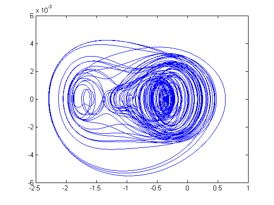
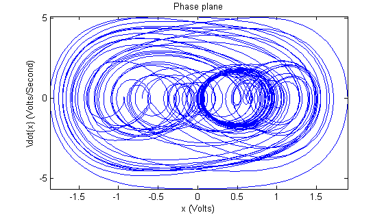
In what follows we present several plots from one of our runs in which we observed chaotic behavior. The plot in FIG. 6 is a time series plot of the voltage measurements collected during the run. One magnetic well is located at around <math>-.4 V</math> (on the ''y''-axis) and the other is at around <math>-1.8 V</math>. One can see that the motions of the tip are highly irregular and indeed appear random. We then passed this data through a Butterworth filter to clean up the high-frequency noise in the signal. The resulting data was then numerically differentiated (we simply used the difference quotients <math>\frac{f(x+h)-f(x)}{h}</math> since our time steps <math>h</math> were extremely small, namely ten-thousandths of a second). Then we plotted the smoothed signal versus its derivative to obtain the picture of the trajectory in phase space (<math>x\text{ vs. }\dot{x}</math>), which is shown in FIG. 7. The Poincaré section in FIG. 8 is obtained from the data plotted in FIG. 7 by plotting one point per oscillation of the motor. The motor was oscillating at 4 Hz and we were sampling at 10,000 Hz so we plotted only the first of every 2,500 data points. The points were then colored to indicate the sequence in which they were plotted. | |||
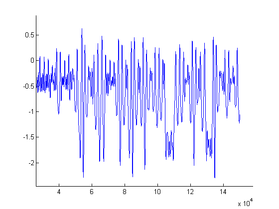
[[Image: | <blockquote><blockquote>[[Image:2100count_4Hz_TimeSeries.png|frame|none|alt=image]] | ||
{Chaotic behavior for sinusoidal forcing of amplitude .0126 m at 4Hz. ''y''-axis units are Volts, ''x''-axis units are (<math>\frac{1}{10,000}</math>)ths of a second} | |||
</blockquote></blockquote> | |||
<blockquote><blockquote>[[Image:2100count_4Hz_PhasePlot.png|frame|none|alt=image]] | |||
{Chaotic behavior for sinusoidal forcing of amplitude .0126 m at 4Hz. ''y''-axis units are Volts per second, ''x''-axis units are Volts} | |||
</blockquote></blockquote> | |||
<blockquote><blockquote>[[Image:2100count_4Hz_PoincareColored.png|frame|none|alt=image]] | |||
We do not | {Poincaré section of trajectory in FIG. 7. Sinusoidal forcing of amplitude .0126 m at 4Hz. ''y''-axis units are Volts per second, ''x''-axis units are Volts. The color indicates the order in which the points were plotted.} | ||
</blockquote></blockquote> | |||
== Attractor Reconstruction. Estimating the Largest Lyapunov Exponent. == | |||
We followed the method outlined in Fraser and Swinney for reconstructing attractors from time series. We use the time series <math>X(t)</math> from our chaotic trial whose graph is shown in FIG. 6 and we plot <math>t\mapsto (X(t), X(t+\tau), X(t+2\tau))</math>, where <math>\tau</math> is chosen to be the first local minimum of the mutual information (see FIG. 9) for <math>(X(t), X(t+\tau))</math>. We do not have the space here to explain this concept in detail, but, heuristically, we want <math>X(t)</math> and <math>X(t+\tau)</math> to be as statistically independent as possible. The 3-dimensional embedding of the reconstructed attractor which results is shown in FIG. 10. | |||
<blockquote><blockquote>[[Image:miMinimization.png|frame|none|alt=image]] | |||
{Minimizing the Mutual Information} | |||
</blockquote></blockquote> | |||
<blockquote><blockquote>[[Image:3dReconstructedAttractor.png|frame|none|alt=image]] | |||
{The reconstructed attractor. The units for each axis are Volts.} | |||
</blockquote></blockquote> | |||
Using the reconstructed attractor plot, we then followed the method in Rosenstein et. al. for estimating the largest Lyapunov exponent. We use an algorithm to find the nearest neighbor of each point on the reconstructed attractor, breaking our time series into a set of closest pairs of points. Then letting <math>d_{j}(i)</math> denote the distance between the <math>j</math>th pair of nearest neighbors at time <math>i\Delta t</math>, we plot the line <math>y(i)=\frac{1}{\Delta t}\langle \ln d_{j}\rangle</math>, where <math>\langle\cdot \rangle</math> is the average over ''j''. The largest Lyapunov exponent is then given by the slope of the least squares fit to this line. | |||
With this method, we found the largest Lyapunov exponent to be .0196 - which is positive, as we would expect for a system exhibiting chaotic behavior (see FIG. 11 above). | |||
<blockquote><blockquote>[[Image:lyapunovExponent.png|frame|none|alt=image]] | |||
{Plot of <math>\frac{1}{\Delta t}\langle \ln d_{j}(i) \rangle</math> (on the ''y''-axis) versus <math>i</math> (on the ''x''-axis). The slope of the least-squares fit line gives us an estimate of the largest Lyapunov exponent.} | |||
</blockquote></blockquote> | |||
= Discussion = | |||
The phase plots of the simulations run with the parameters estimated in III.B are shown in FIG. 12, FIG. 13, and FIG. 14 below. | |||
<blockquote><blockquote>[[Image:simulation_leftWell_params_phasePlot.png|frame|none|alt=image]] | |||
{The plot in phase space of the simulation starting from <math>(-.7,0)</math>, using the parameters obtained from the ``small ''f''" oscillations in the right well.} | |||
</blockquote></blockquote> | |||
<blockquote><blockquote>[[Image:simulation_rightWell_params_phasePlot.png|frame|none|alt=image]] | |||
{The plot in phase space of the simulation starting from <math>(-.7,0)</math>, using the parameters obtained from the ``small ''f''" oscillations in the left well.} | |||
</blockquote></blockquote> | |||
<blockquote><blockquote>[[Image:simulation_averageWell_params_phasePlot.png|frame|none|alt=image]] | |||
{The plot in phase space of the simulation starting from <math>(-.7,0)</math>, using the parameters obtained from the average of ``small ''f''" oscillations in the left and right wells.} | |||
</blockquote></blockquote> | |||
Compare these plots to that of the one we were attempting to simulate (shown in FIG. 7) and you will notice several significant discrepancies. For one thing, only the simulation using the ``right well" parameters showed any significant chaotic behavior, and even in that case the chaotic transient ended fairly quickly in a limit cycle. None of these plots had enough chaotic behavior to generate any meaningful Poincaré section or to use the method of Lyapunov exponent estimation via attractor reconstruction. | |||
The other fact that needs to be pointed out is that the experimental plot in FIG. 7 is extremely asymmetric (the trajectories spending a disproportionately long time in the right well, which is apparently much larger than the left well). The simulation plots, on the other hand, are quite symmetric. We believe this asymmetry is due to the natural bend of the shim stock in the direction of the magnet corresponding to the right-hand potential well. There are also noticeable differences in the strength of the magnets, which certainly contributes to this observed asymmetry as well. | |||
= Conclusion = | |||
We must acknowledge that the forced Duffing oscillator is now something of a classical example of a chaotic dynamical system, and it has been thoroughly studied in theory and experiment. Although we did not necessarily do anything new, we found it to be a very deep and complicated system. It was a great chance to apply the theory which was presented in the class. In the course of our experiment and analysis we learned about a number of interesting and fruitful techniques for the study of chaotic dynamics. | |||
We still have number of questions regarding the Duffing oscillator and our experiment which we find very interesting. We would like to explore several different directions in the future. In particular, we would like to analyze forced oscillators with asymmetric potential wells, which can be modeled by setting <math>V(x)= \frac{\beta }{4}x^{4}+\frac{\epsilon_{1}}{3}x^{3}-\frac{\alpha}{2} x^{2}+\epsilon_{2}x</math>. We would also like to study the case of nonsinusoidal periodic forcing, where we replace <math>\cos</math> with some other function <math>\rho(\omega t)</math> which is possibly piecewise smooth (or merely piecewise <math>C^{\alpha}(\mathbb{R})</math>). Exploring either of these questions will require further refining the experimental setup, continued study of numerical simulations, and some new mathematical/theoretical techniques. | |||
= References = | = References = | ||
Revision as of 08:55, 14 December 2012
Group members: Ross Granowski, Aemen Lodhi, Andrew Champion, Suchithra Ravi

We compare a mechanically forced double-well Duffing oscillator with an asymmetric potential to numeric simulations of a symmetric potential system. Analysis is performed with time series data, phase portraits, recurrent Poincare sections, attractor reconstruction from time delay embedding, and Lyapunov exponent estimation from this reconstruction. Our investigation finds that the asymmetric mechanical system can exhibit chaos while for the same forcing parameters symmetric simulation produces limit cycles above or below the chaotic threshold depending on the mechanical potential well used to estimate simulation parameters.
Introduction
The forced Duffing oscillator is a seminal system for the study of chaotic dynamics and development of analytical and experimental techniques for nonlinear systems. A common physical interpretation for the double-well case of the Duffing oscillator model considered here is a ferromagnetic beam positioned between two magnets while undergoing lateral forcing, as illustrated in Figure~\ref{fig:beam_illustration}. This mechanical system elucidates several features of the model Duffing oscillator: a potential for the lateral position of the beam created by the two magnets; non-autonomous forcing resulting in motion of the beam, potentially chaotically between the two wells; and mechanical dissipation within the beam and from air resistance against the beam's motion.
Though the Duffing oscillator and the double-well beam system are simple and not of any obvious utility in their own right, they provide a structured model with few, well-defined parameters and clear physical interpretations while still producing chaotic dynamics. This allows intuition into the system's behavior and creates an accessible and familiar setting for experimental design, data analysis, and diagnosis of unexpected results. All these features are valuable both for pedagogical purposes and for the development of new methods and tools for analysis, experimentation, computation, and diagnosis that may be extensible to more complex systems or other scientific or engineering applications.
The periodically-forced Duffing oscillator is a system governed by the following nonlinear and nonautonomous second-order ODE (``The Duffing Equation"): <math>\ddot{x}+\delta \dot{x}-\alpha x+\beta x^{3}=f \cos(\omega t)</math> for constants <math>\alpha,\beta,\delta,\omega,f>0</math>. Although it can be viewed as a planar (2 dimensional) system, the nonautonomous periodic term <math>f \cos(\omega t)</math> means that the equation actually determines a smooth vector field on <math>\mathbb{R}^{2}\times \mathbb{S}^{1}</math> (a 3 dimensional space) and hence truly chaotic behavior is possible.
To begin to understand this equation, it is simplest to first analyze the case where <math>\delta=f=0</math>. In this case our equation reduces to <math>\ddot{x}-\alpha x+\beta x^{3}=0</math> which is a Newtonian system with potential <math>V(x)= \frac{\beta }{4}x^{4}-\frac{\alpha}{2} x^{2}</math> and the trajectories are curves of constant energy <math>E(x,\dot{x})=\frac{1}{2}\dot{x}^{2}+V(x)</math>. In this case it is easy to see that we have a saddle at the origin and centers at <math>\left(\pm\sqrt{\frac{\alpha}{\beta}},0\right)</math>. Other than the two homoclinic orbits from the origin to itself and the two centers, we have that all other trajectories are in fact closed orbits.
Now when we include the dissipation term (i.e. we let <math>\delta>0</math>), the system is again easy to understand: heuristically, trajectories spiral into what are now stable fixed points at <math>\left(\pm\sqrt{\frac{\alpha}{\beta}},0\right)</math>. We can see that in this case <math>\frac{d}{dt}E = \dot{x}(\ddot{x}+\beta x^{3}-\alpha x)=-\delta\dot{x}^{2}\leq 0</math> so the energy decreases (strictly, when <math>\dot{x}\neq 0</math>) along trajectories of the system. The origin is still a saddle in this case. It can be shown that, except for the stable manifolds of the saddle, all trajectories of this system tend toward one of the stable fixed points.
When we let <math>f>0</math>, the behavior of the system becomes quite complicated. For sufficiently small values of f we find that we have stable limit cycles near what were stable fixed points for <math>f=0</math>, and almost all trajectories eventually converge to one of the two limit cycles (namely all except for the measure zero stable manifolds of the saddle point at the origin). For very large f, it can be shown there is one globally stable limit cycle attracting all trajectories. For intermediate values of f, however, we have chaotic behavior of trajectories in phase space. This is essentially due to the fact that as we increase f from 0, we eventually cause the stable and unstable manifolds of the saddle at <math>(0,0)</math> to intersect, and hence to intersect infinitely many times. The presence of infinitely many homoclinic intersection points in (a compact region of) phase space causes the trajectories to have very complex topological structures. These can be seen most clearly via the Poincaré section (sampling the orbit at time intervals of length <math>\frac{2\pi}{\omega}</math>), which displays intricatre fractal ``strange attractors" for these chaotic values of f.
In our experiment, we constructed a mechanical system whose behavior is approximately governed by the above equation. In essence, we used two magnets placed symmetrically about the tip of a strip of shim stock to give us a system behaving like <math>\ddot{x}=-\delta \dot{x}+\alpha x-\beta x^{3}</math>. Here x denotes the displacement of the tip of the stock, with the vertical beam giving us x=0 and the magnets being located at <math>\pm\sqrt{\frac{\alpha}{\beta}}</math>. We can think of the tip of the stock as a particle trapped in a ``double well" potential. We then used a motor to generate the periodic forcing by shaking the apparatus in the lateral direction.
Our apparatus was modeled on that of Moon and Holmes , where they use essentially the same setup (although inverted - which we are assuming makes almost no difference, since gravity never appears in any of the ``governing equations"). In the Moon and Holmes paper, they show that the Duffing equation is indeed a good model for this system via a clever reduction (using Galerkin’s method) of a system of PDEs. This analysis, although interesting, is somewhat complicated and does not significantly improve our intuition for the system, so we refer the interested reader to the Moon and Holmes paper for further details. Indeed, the readers seeking a more detailed mathematical analysis of this system should conslult the papers of Holmes and Moon and Holmes.
Our goal at the outset was to analyze the bifurcations of the physical system in the <math>(f,\omega)</math> plane for fixed values <math>\alpha,\beta,\delta</math>. We state here that the Duffing equation is already nondimensionalized. Later, we will use our experimental results to approximate the values of <math>\alpha, \beta, \delta</math> appearing in the eqation. We the run computer simulations with these parameters and compare them to our data.
Methods
Experimental Setup
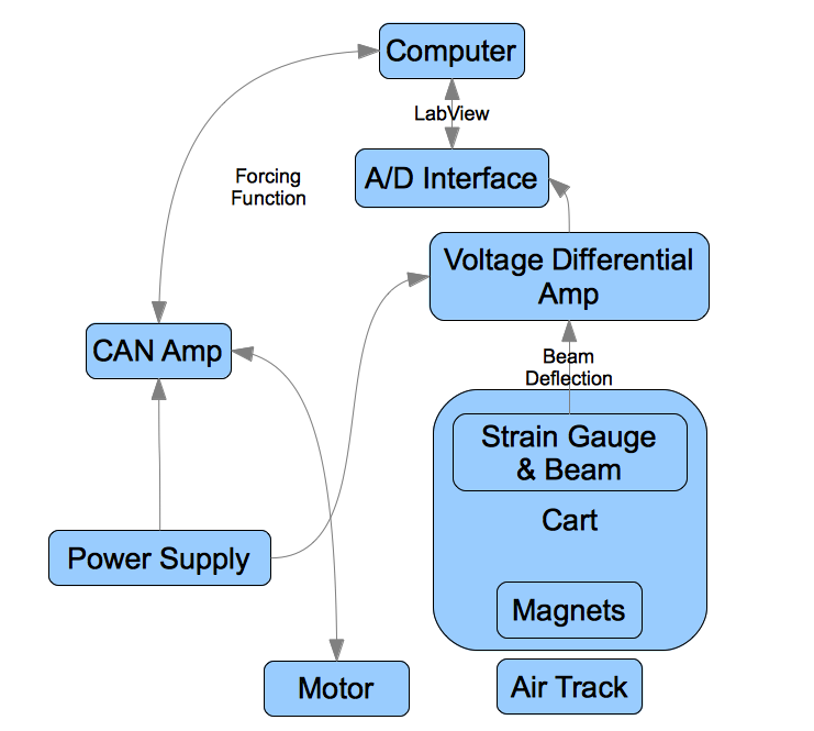
{Components and Connection of Experimental Apparatus}

For the mechanical system itself (the source of the data), we attached a slender metallic beam to a rigid frame made from 80/20. The beam was cut from shim stock of thickness .007 inches (.0001778 m). Although we had originally planned to use electromagnets, we would have had to weight the end of the beam in order to produce the desired buckling behavior. Weighting the stock correctly proved rather difficult, so insead we used very powerful stationary magnets and an unweighted beam. Two rare earth magnets were attached symmetrically to the top of the frame. The strength of the magnets was such that the metallic beam always buckled in the direction of one of magnets, with either configuration (being buckled to the left or to the right) constituting a stable equilibrium. The position of the beam in the center is an unstable equilibrium. Since the focus of this experiment was on understanding the forced vibrations of the beam, we then applied an external force to the entire framework with a motor whose position was controlled through the computer.
We note here that for controlling the motion of the motor we specified the frequency (in Hz – generally 3, 4, or 5 Hz – although we wrote a program in LabView which allowed us to generate motion at arbitrary frequencies), the forcing function (a sine wave), and the amplitude of oscillation. The amplitude of oscillation was measured in terms of ``counts," where 1000 counts = .006 m.
To measure the displacement of the tip, we decided to use strain gauges, which were attached near base of beam. The strain gauges – essentially a type of variable resistor – were used to create a voltage differential which was then amplified and sent to the computer where it was plotted as a function of time. Our sampling rate here was 10,000 Hz (i.e. we recorded 10,000 voltage measurements per second). The strain gauges are basically measuring the local deflection at the base of the beam (in the immediate vicinity of the strain gauge). Thus we worried that the resulting voltage measurements would not be adequate, since we are really just concerned with the position of the tip of the beam. We had originally inteded to use a webcam as well, but we found that the strain gauges actually had good accuracy and precision, minimal drift, and adequate range. Hence a camera was not needed. Measuring the tip position versus voltage reading, we found an approximate linear correspondence between voltage and distance: 1.4V corresponds to approximately .045 m.
A conceptual schematic of the experimental setup is presented in FIG. 1, above.
Evolution of the Apparatus
This apparatus went through several iterations as we attempted to correct various problems and improve the design.
{First Iteration of the Setup}
For the first iteration (see FIG. 2) we had a wheeled cart on a low-friction track (borrowed from the undergraduate Physics I lab). The cart carried the 80/20 frame and we held the motor stationary and attached the motor arm to the cart. There measurement setup was fine, but there were several mechanical problems with this setup: the motor was difficult to attach to the cart and there was a problematic amount of friction coming from the wheels of the cart (the weight of the frame on top was causing a wheel to ``stick").
{Second Iteration of the Setup}
For the second iteration (see FIG 3) we replaced the cart and track with an air track. This time we held the motor arm stationary while attaching the frame to the top of the motor. This was a significant improvement over the first iteration (basicallly eliminating the friction problem). But we still had several problems: most importantly, the shim stock would strike the frame when its motion became chaotic. For large amplitudes and/or frequencies of oscillation, this setup would also cause intense vibrations of the table and the entire apparatus.
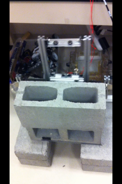
{Third Iteration of the Setup}

For the third and final iteration (see FIG 4) we addressed these problems by widening the 80/20 frame to accomodate chaotic motion and we mounted the apparatus on cinderblocks which were adhered to the floor and to one another. We still have problems with this setup, however. There are problems with effectively cooling the motor and the CAN amplifier. The motor’s current limitiations are also preventing us from driving the system hard enough to observe sustained chaotic motion. There is also the issue of asymmetry in the system due to a difference in magnet strength and the natural bend in the stock, neither of which have we been able to effectively eliminate or compensate for. This is apparent in our data below.
Results
Parameter Estimation
Following Berger and Nunes, we estimate the values of <math>\alpha, \beta,\text{ and }\delta</math> appearing in the Duffing equation using our experimental data. We will then use these estimated values (together with the known values of f and <math>\omega</math>) in a computer simulation, which we compare to the results of a particular trial.
According to our data, we have fixed points at approximately <math>\pm\sqrt{\frac{\alpha}{\beta}}\approx \pm .7 V</math> (the strain gauges would shift over time, but this is the position once we normalize by subtracting the mean from the data). Writing <math>x(t)=-\sqrt{\frac{\alpha}{\beta}}+\phi(t)</math>, substituting this into the Duffing equation and ignoring the forcing term, we find that to first order in <math>\phi</math> we have <math>\ddot{\phi}(t)=-\delta\dot{\phi}(t)-2\alpha\phi(t)</math>. We know that this gives us damped simple harmonic motion with frequency <math>\omega_{1}=\sqrt{2\alpha(1-\delta^{2}/8\alpha)}</math>. Solving in terms of <math>\delta</math> gives us <math>\delta =\sqrt{8\alpha(1-\omega_{1}^{2}/2\alpha)}</math>. From our experimental data we get an approximate value for <math>\omega_{1}</math> (based on the period of oscillation in the small amplitude case) and guess <math>\alpha</math> such that <math>\omega_{0}=\sqrt{2\alpha}</math> is only slightly larger than <math>\omega_{1}</math>.
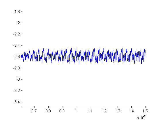
{A ``small f" limit cycle, y-axis units are Volts, x-axis units are (<math>\frac{1}{10,000}</math>)ths of a second}

From a set of data where the stock remained oscillating with low amplitude in the right well (time series pictured in FIG. 5 above), we found that <math>\omega_{1,\text{left}}=2.0\text{cycles/second}</math>. Thus we have <math>\beta=\frac{\alpha}{.49}</math> and <math>\delta= \sqrt{8\alpha(1-2/\alpha)}</math>. We observed chaotic behavior for forcing with amplitude 2100 count (so approximately .392 V, using .006 m per count and 1.4V per .045m) and frequency 4Hz so <math>f=\text{amplitude}*\text{frequency}^{2}\approx 6.272</math>. Setting <math>\alpha=2.01</math> is physically reasonable, since then <math>\omega_{0}=\sqrt{2\alpha}\approx 2.004</math> is the undamped frequency (this should be just a little bigger than the damped frequency <math>\omega_{1,\text{left}}</math>). For the left well we find <math>\omega_{1_\text{right}}=4.76\text{cycles/sec}</math>. Again <math>\beta=\frac{\alpha}{.49}</math> and now <math>\delta= \sqrt{8\alpha(1-22.6576/2\alpha)}</math>. In this case (for our simulation) we set <math>\alpha=11.33</math> (which gives us <math>\omega_{0}\approx 4.7602</math>).Averaging the two values of <math>\omega_{1}</math> we get <math>\omega_{1, \text{avg}}=3.38</math>. Again <math>\beta=\frac{\alpha}{.49}</math> and now <math>\delta= \sqrt{8\alpha(1-11.424/2\alpha)}</math>. Now for our simulation with these parameters we set <math>\alpha=5.714</math> (which gives us <math>\omega_{0}\approx 3.3805</math>). {Plots}
In what follows we present several plots from one of our runs in which we observed chaotic behavior. The plot in FIG. 6 is a time series plot of the voltage measurements collected during the run. One magnetic well is located at around <math>-.4 V</math> (on the y-axis) and the other is at around <math>-1.8 V</math>. One can see that the motions of the tip are highly irregular and indeed appear random. We then passed this data through a Butterworth filter to clean up the high-frequency noise in the signal. The resulting data was then numerically differentiated (we simply used the difference quotients <math>\frac{f(x+h)-f(x)}{h}</math> since our time steps <math>h</math> were extremely small, namely ten-thousandths of a second). Then we plotted the smoothed signal versus its derivative to obtain the picture of the trajectory in phase space (<math>x\text{ vs. }\dot{x}</math>), which is shown in FIG. 7. The Poincaré section in FIG. 8 is obtained from the data plotted in FIG. 7 by plotting one point per oscillation of the motor. The motor was oscillating at 4 Hz and we were sampling at 10,000 Hz so we plotted only the first of every 2,500 data points. The points were then colored to indicate the sequence in which they were plotted.
{Chaotic behavior for sinusoidal forcing of amplitude .0126 m at 4Hz. y-axis units are Volts, x-axis units are (<math>\frac{1}{10,000}</math>)ths of a second}

{Chaotic behavior for sinusoidal forcing of amplitude .0126 m at 4Hz. y-axis units are Volts per second, x-axis units are Volts}

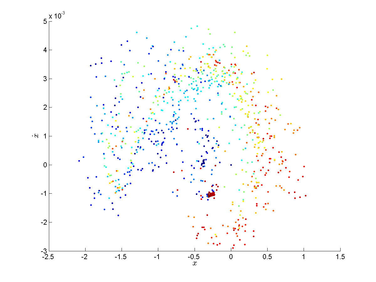
{Poincaré section of trajectory in FIG. 7. Sinusoidal forcing of amplitude .0126 m at 4Hz. y-axis units are Volts per second, x-axis units are Volts. The color indicates the order in which the points were plotted.}

Attractor Reconstruction. Estimating the Largest Lyapunov Exponent.
We followed the method outlined in Fraser and Swinney for reconstructing attractors from time series. We use the time series <math>X(t)</math> from our chaotic trial whose graph is shown in FIG. 6 and we plot <math>t\mapsto (X(t), X(t+\tau), X(t+2\tau))</math>, where <math>\tau</math> is chosen to be the first local minimum of the mutual information (see FIG. 9) for <math>(X(t), X(t+\tau))</math>. We do not have the space here to explain this concept in detail, but, heuristically, we want <math>X(t)</math> and <math>X(t+\tau)</math> to be as statistically independent as possible. The 3-dimensional embedding of the reconstructed attractor which results is shown in FIG. 10.
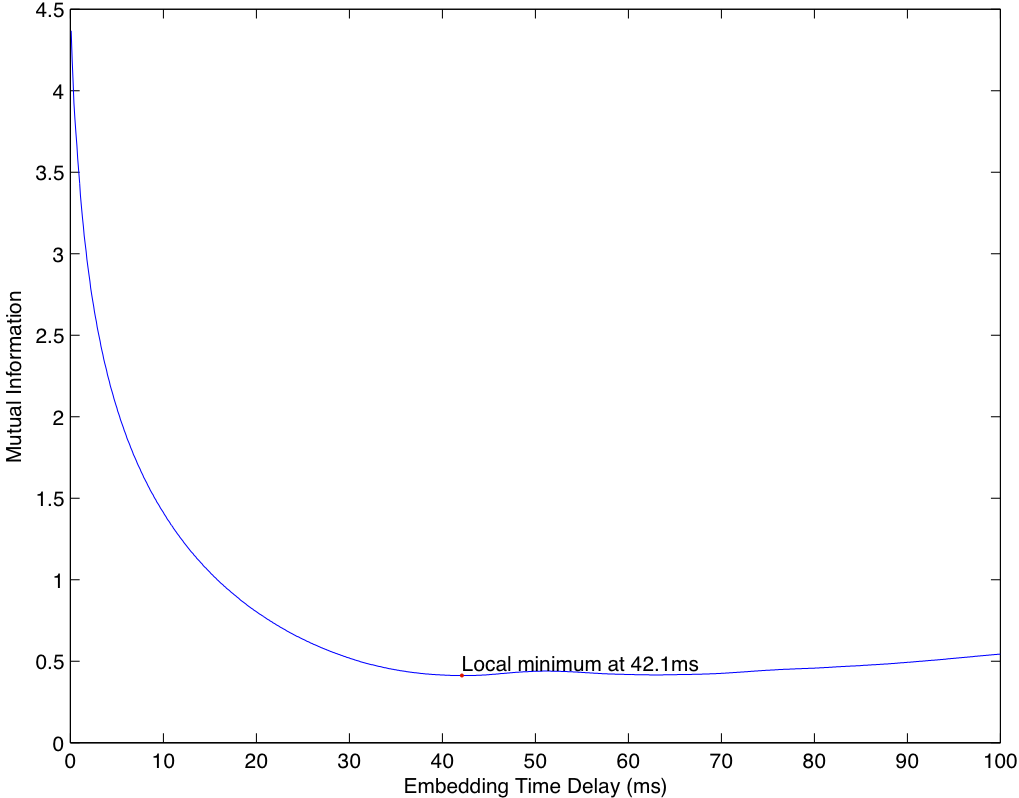
{Minimizing the Mutual Information}

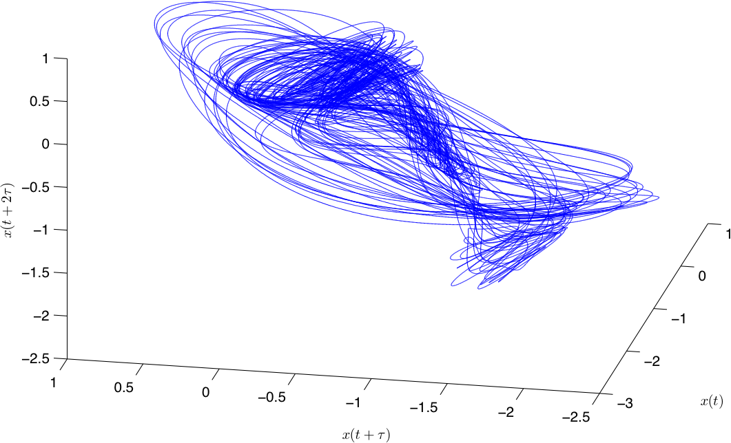
{The reconstructed attractor. The units for each axis are Volts.}

Using the reconstructed attractor plot, we then followed the method in Rosenstein et. al. for estimating the largest Lyapunov exponent. We use an algorithm to find the nearest neighbor of each point on the reconstructed attractor, breaking our time series into a set of closest pairs of points. Then letting <math>d_{j}(i)</math> denote the distance between the <math>j</math>th pair of nearest neighbors at time <math>i\Delta t</math>, we plot the line <math>y(i)=\frac{1}{\Delta t}\langle \ln d_{j}\rangle</math>, where <math>\langle\cdot \rangle</math> is the average over j. The largest Lyapunov exponent is then given by the slope of the least squares fit to this line.
With this method, we found the largest Lyapunov exponent to be .0196 - which is positive, as we would expect for a system exhibiting chaotic behavior (see FIG. 11 above).
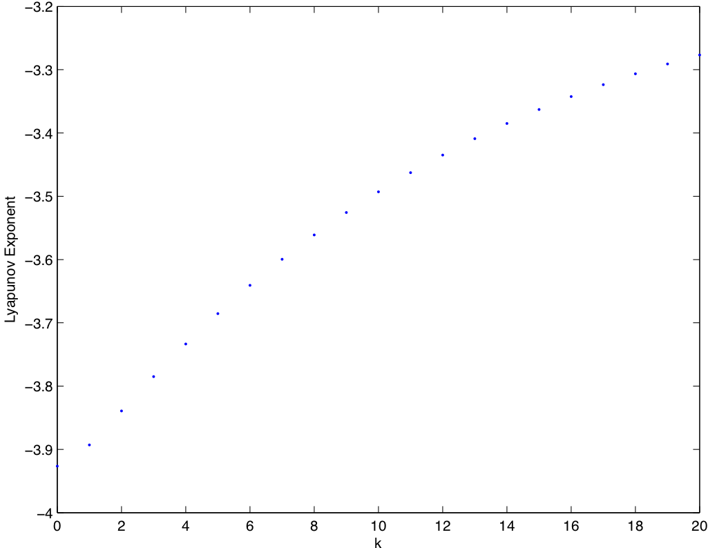
{Plot of <math>\frac{1}{\Delta t}\langle \ln d_{j}(i) \rangle</math> (on the y-axis) versus <math>i</math> (on the x-axis). The slope of the least-squares fit line gives us an estimate of the largest Lyapunov exponent.}

Discussion
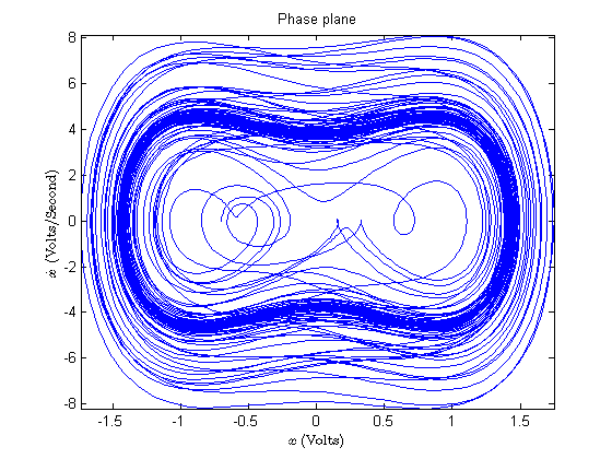
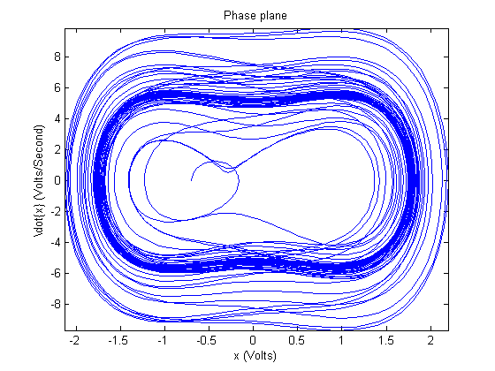
The phase plots of the simulations run with the parameters estimated in III.B are shown in FIG. 12, FIG. 13, and FIG. 14 below.
{The plot in phase space of the simulation starting from <math>(-.7,0)</math>, using the parameters obtained from the ``small f" oscillations in the right well.}

{The plot in phase space of the simulation starting from <math>(-.7,0)</math>, using the parameters obtained from the ``small f" oscillations in the left well.}

{The plot in phase space of the simulation starting from <math>(-.7,0)</math>, using the parameters obtained from the average of ``small f" oscillations in the left and right wells.}

![[1]](http://en.wikipedia.org/wiki/File:Tw_duffing.png)
Compare these plots to that of the one we were attempting to simulate (shown in FIG. 7) and you will notice several significant discrepancies. For one thing, only the simulation using the ``right well" parameters showed any significant chaotic behavior, and even in that case the chaotic transient ended fairly quickly in a limit cycle. None of these plots had enough chaotic behavior to generate any meaningful Poincaré section or to use the method of Lyapunov exponent estimation via attractor reconstruction.
The other fact that needs to be pointed out is that the experimental plot in FIG. 7 is extremely asymmetric (the trajectories spending a disproportionately long time in the right well, which is apparently much larger than the left well). The simulation plots, on the other hand, are quite symmetric. We believe this asymmetry is due to the natural bend of the shim stock in the direction of the magnet corresponding to the right-hand potential well. There are also noticeable differences in the strength of the magnets, which certainly contributes to this observed asymmetry as well.
Conclusion
We must acknowledge that the forced Duffing oscillator is now something of a classical example of a chaotic dynamical system, and it has been thoroughly studied in theory and experiment. Although we did not necessarily do anything new, we found it to be a very deep and complicated system. It was a great chance to apply the theory which was presented in the class. In the course of our experiment and analysis we learned about a number of interesting and fruitful techniques for the study of chaotic dynamics.
We still have number of questions regarding the Duffing oscillator and our experiment which we find very interesting. We would like to explore several different directions in the future. In particular, we would like to analyze forced oscillators with asymmetric potential wells, which can be modeled by setting <math>V(x)= \frac{\beta }{4}x^{4}+\frac{\epsilon_{1}}{3}x^{3}-\frac{\alpha}{2} x^{2}+\epsilon_{2}x</math>. We would also like to study the case of nonsinusoidal periodic forcing, where we replace <math>\cos</math> with some other function <math>\rho(\omega t)</math> which is possibly piecewise smooth (or merely piecewise <math>C^{\alpha}(\mathbb{R})</math>). Exploring either of these questions will require further refining the experimental setup, continued study of numerical simulations, and some new mathematical/theoretical techniques.
References
<references> <ref name="GuckenheimerHolmes">Guckenheimer, J. and P. Holmes (1983). Nonlinear Oscillations, Dynamical Systems, and Bifurcations of Vector Fields. Springer-Verlag.</ref> <ref name="Holmes">Holmes, P. (1979). A nonlinear oscillator with a strange attractor. Phil. Trans. R. Soc. Lond. A 292, 419–448.</ref> <ref name="Morozov">Morozov, A. (1973). Approach to a complete qualitative study of duffing’s equation. USSR Comput. Math. math. Phys. 13(5), 45–66.</ref> <ref name="VariousPeriodicForces">Ravichandran, V., V. Chinnathambi, and S. Rajasekar (2006). Effect of various periodic forces on duffing oscillator. Pramana 67(2), 351–356.</ref> </references>