Group 7: Difference between revisions
No edit summary |
|||
| Line 4: | Line 4: | ||
== Background == | == Background == | ||
== Linear Stability Analysis == | == Linear Stability Analysis == | ||
Revision as of 21:23, 7 December 2011
Group Members: J. J. Aguiliar, G. Lee, C. Marcotte, B. Suri
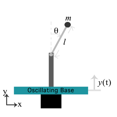
The inverted pendulum is a simple mechanical system which models a canonical problem in both Control Theory and Nonlinear Dynamics. It is possible to control this system through either horizontal or vertical control of the pivot point. This article explores control of the planar pendulum through oscillation of the vertical position of the pivot point.
Background
Linear Stability Analysis
Clearly, the fixed points are given by $(\theta^{*}, \dot{\theta^{*}})_{-} = (\pi,0)$ and $(\theta^{*}, \dot{\theta^{*}})_{+} = (0,0)$. Making the local transformation $\eta_{\pm} = \theta^{*}_{\pm} + \delta\theta_{\pm}$ we derive the Mathieu equations.<ref name = Bartuccelli></ref>
\begin{equation}
\delta\ddot{\theta}_{\pm} \pm (\beta f(\tau) - \alpha)\delta\theta_{\pm} = 0
\end{equation}
Note that the stability of the fixed point is determined by the sign of the linear prefactor, and that, should $y(t)$ be an eigensolution of the operator $\partial^{2}_{\tau}$ with eigenvalue $-1$, that the stability of the fixed points are not determined by the sign of $\beta$ as $-\beta$ corresponds to a phase shift of $\pi$ relative to $\beta$.
Experiment
Through the use of a motor we attempt to force the stability of the free pendulum, such that the downward vertical $(\theta^{*}_{-} = \pi)$ becomes unstable and the upward vertical $(\theta^{*}_{+} = 0)$ becomes stable. We intend to investigate extending this to the case of coupled (series) pendula. We assume the limit $\gamma \rightarrow 0$.
Materials
- Motor or shaking table
- Rod or Pendulum Simulacrum
- Reflective Tracking Tape
- Camera
- Matlab, no doubt
Simulation
A simulation was construction based on the single inverted pendulum model with a vertically oscillating pivot. The simulation was done through Matlab with Simulink. The equations of motion for such a model reduce to the following equation:
\begin{equation} \ddot{ \theta} = \sin(\theta)\cdot(g/l - \ddot{y}/l) \end{equation}
where $\theta$ is the angular position of the rod, $g$ is gravity, and $l$ is the rod length. And for a vertical forcing of the following form: $y(t) = A\sin(\omega t)$, the resulting equation used in the model is the following:
\begin{equation} \ddot{ \theta} = \sin(\theta)(g/l-(A/l)\omega^2\cdot\sin(wt)) \end{equation}
where $A$ and $\omega$ are the amplitude and angular frequency, respectively.
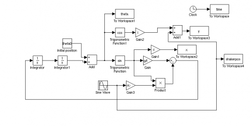
Based on these equations, the following Simulink model was created.
This model is a block diagram representation of the equation of motion formulated above. At the first time step, $t=0$, it uses an initial angular position of the rod to calculate the angular acceleration and then integrates twice into the next time step as the shaker also moves to its next position in time. The output is an array of angular positions in time, which can be transformed to their appropriate x and y positions.
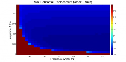
With this model, one can easily vary the shaker frequency and amplitude and observe the pendulum’s behavior for different values. For example, a useful metric easily attainable with this model is the range of the horizontal bounds of the pendulum’s trajectory, or xmax - xmin. The following figure is a sample result of the horizontal range for 10 cm long rod starting at $\theta_o = \pi/30$ for a sweep of frequencies and amplitudes.
Notice that there is a point when the range jumps to 0.2 m (twice the rod length). This indicates that the pendulum was not able to exhibit a stable oscillation about the vertical fixed point and instead fell. Keeping the amplitude constant and sweeping only through frequencies, one can observe how the critical stabilization frequency would vary as the initial angular position changes.
Expectations
<videoflash>8S3Ylw7ukJ0</videoflash>
Given the above, it would seem possible to stabilize the double and triple inverted pendulum. So we expect, for carefully determined parameter values, that such stability can be attained for the single inverted pendulum. It may be the case that unbounded $\theta$ requires an initial transient to nudge the pendulum into the stable domain.
References
<references/>


