Group 3
Inelastic bouncing ball
Group members: Nitin Arora, Phillip Gray, Chris Rodesney, Jacob Yunis
Presentation. Papers: Nitin, Phillip, Jacob, Chris

The appropriately-named bouncing inelastic ball experiment is composed of a perfectly inelastic ball bouncing on an oscillating plate. It is a simple yet elegant system that exhibits striking nonlinear behavior. On this page, we construct a computational model using various forcing waveforms for the plate, and generate associated bifurcation diagrams. We also explore experimentally the case of a harmonically forced plate.
Theory
The system of a ball bouncing completely inelastically on a vibrated platform has been the subject of numerous studies <ref>A. Mehta and J. M. Luck, Physical Review Letters 65, 393 (1990)</ref> <ref>T. Gilet, N. Vandewalle, and S. Dorbolo, Physical Review E 79, 055201(R) (2009)</ref>, and the case of a simple harmonically vibrated plate was completely resolved by Gilet et al. The primary means for analyzing the motion is measuring the time of flight between successive impacts of the ball with an n-cycle corresponding to the ball having n unique flight times before repeating. For small forcing, Gilet et al found an alternating series of one and two cycles with a small region containing an infinity of bifurcations around control parameter $\Gamma \simeq 7.253378$.
We investigate the case of a plate vibrated according to a superposition of two sine waves with a frequency ratio $c$:
<math> \begin{equation} x_p(t) = A[\sin(\omega t) + \sin(c \omega t)] \end{equation} </math>
The ball can take off from the plate when the acceleration of the plate is less than negative g, the acceleration due to gravity:
<math> \begin{align} \ddot{x}_p(t) = -A[\omega^2\sin(\omega t) + c^2 \omega^2\sin(c \omega t)] &\leq -g \notag\\ \frac{A\omega^2}{g} [\sin(\omega t) + c^2 \sin(c \omega t)] &\geq 1 \end{align} </math>
In this way, the motion of the ball from initial takeoff at <math>t_0</math> is:
<math> \begin{align} x_b(t) = &x_p(t_0) - x_p(t) + \dot{x}_p(t_0)(t-t_0) - 1/2 g(t-t_0)^2 \notag\\ x_b(t) = &A[\sin(\omega t_0)+ \sin(c \omega t_0) - \sin(\omega t) - \sin(c \omega t)] + A[\omega \cos(\omega t_0) + c \omega \cos(c \omega t_0)](t-t_0) - 1/2 g(t-t_0)^2 \notag \end{align} </math>
<math> \Gamma, \varphi, \chi</math> regime
The above functions can be made dimensionless via the introduction of a characteristic time <math>1/\omega</math> and a characteristic length <math>g/\omega^2</math>. We can thus define a phase <math>\varphi = \omega t</math>, a reduced acceleration and one of our control parameters <math>\Gamma = A\omega^2/g</math>, and a generalized position <math>\chi = A\omega^2/g</math>. The other control parameter is the ratio of the frequencies <math>c</math>.
The forcing of the plate is now given by:
<math> \begin{equation} \chi_p(\varphi) = \Gamma(\sin(\varphi) + \sin(c \varphi)) \end{equation} </math>
The position of the ball relative to the plate is
<math> \begin{align} \chi_b(\varphi) = &\Gamma[\sin(\varphi_0)+ \sin(c \varphi_0) - \sin(\varphi) - \sin(c \varphi)] + \dots \\ &\Gamma[\cos(\varphi_0) + c\cos(c \varphi_0)](\varphi - \varphi_0) - 1/2(\varphi-\varphi_0)^2. \notag \end{align} </math>
and the ball takes off when
<math> \begin{equation} \Gamma [\sin(\varphi) + c^2 \sin(c \varphi)] \geq 1 \end{equation} </math>
Period Doubling and Chaos
The flight time is defined as <math>T = \varphi_i - \varphi_0</math>, and can be found by solving the following equation numerically:
<math> \begin{align} F \equiv &\Gamma [\sin(\varphi_0)(1-\sin T) + \sin(c\varphi_0)(1-\sin cT) - \cos T \cos(\varphi_0) - \cos(cT)\cos(c\varphi_0)] - \dots \\
&\Gamma[\cos(\varphi_0) + c\cos(c\varphi_0)]T - 1/2 T^2 = 0
\end{align} </math>
The ball is able to land in two distinct regions. There is a 'bouncing' region, where the acceleration of the plate is such that the ball will immediately take off again, with an initial velocity equal to the instantaneous velocity of the plate at the time of impact. The other region is the 'sticking' region, where the ball is not able take off, and instead rests on the plate until the plate's acceleration is such that is can take off again. This region is a sort of resetting region, as the ball immediately forgets any history it had prior to landing. The sticking region will mark the boundary between periodic cycles.
By varying the control parameter <math>\Gamma</math> we construct bifurcation diagrams for the cases <math>c=1, c=2</math> and <math>c=3</math>.
Bifurcation Diagrams
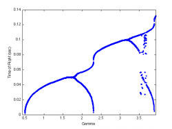
<math>c=1</math>
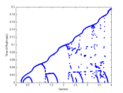
<math>c=2</math>
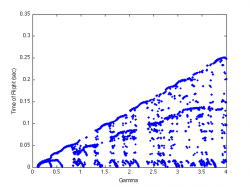
<math>c=3</math>


Parts list
- oscilloscope or computer capable of outputting different forcing functions
- shaker plate
- completely inelastic hacky-sack type ball
- high speed camera with computer interface
- tracking software
Experimental Methods
In order to set up an inelastic bouncing ball system in the lab, we had to overcome 3 primary challenges: using a truly inelastic ball, constraining the ball to 1D motion, and accurately calculating the time of flight.


Initially, a sand filled bag on a driven plate surrounded by a plastic fence was used, see above. An accelerometer in the driven plate was used to calculate flight time. The input sine wave determined the takeoff point by calculating the takeoff line. The input sine wave was then subtracted out of the accelerometer signal to calculate the landing point. This signal was too noisy to be of use and the ball did not consistently remain in the center of the plate.

The lab setup was then reconfigured (see Final Setup above). A metal block ($m = 249 g$) with ball bearings was attached to a vertical pole to stabilize the motion in 1-D. This came at a cost of friction of the mass on the pole and slight elasticity of the mass. The friction was assumed to be Coulomb friction: constant with and opposite in sign to velocity. The friction was observed to be approximately $0.29g$. The takeoff times were calculated using an electrical circuit which was grounded at <math>x = 0 </math> The resulting signal provided very precise takeoff times. The coefficient of restitution of the mass was observed to be <math>c_{R}\approx 0.515</math>.


The friction was incorporated into the computational model developed in the Introduction, however the <math>c_{R}</math> was not, due to time constraints. Other experimental issues include the slight twisted of the mass due to nonuniform impact with the plate and low frequency shaker oscillation cause by feedback from the mass striking the plate at high <math>\Gamma</math>.
Data was collected at a sample rate of 20 KHz. The frequency of the plate was held constant during a run; the amplitude of the plate was altered to produce varying <math>\Gamma</math>. The frequency was varied between 20 and 40 Hz from run to run. The amplitude was stepped up gradually from <math>\Gamma=0</math> to <math>\Gamma=8</math> using a constant stepwise function. Different strategies were used to try to limit transients in the dynamics due to changing <math>\Gamma</math>. The optimal setup was to examine small ranges of <math>\Gamma</math> at a time, with between <math>50</math> and <math>100</math> oscillations at each <math>\Gamma</math>. In addition, the first <math>10</math> oscillations at each $\Gamma$ thrown out to allow the system to settle.

Data Acquisition
Data acquisition was handled using Lab View software. Data was recorded at 20 KHz in two channels; plate acceleration and voltage from the continuity sensor. The data was output from Labview in a tab delimited format with four columns. An additional column was added to the data containing the time stamp for each measurement. The Figure 6 shows a block diagram of the informational flow.

LabView was used to control the vibrating plate. LabView output the driving signal oscillating between -2.5 and 2.5 V. The signal was then passed through an amplifier whose gain was adjusted such that the minimum and maximum accelerations desired could be achieved. Data was taken by continuously increasing the amplitude of the voltage applied to the shaker table such that the acceleration slowly increased from 0g to 8g. Physically, this adjusted $\Gamma$ by increasing the amplitude of vibration while maintaining a constant frequency. This was done in steps where a constant maximum amplitude was held for a specified number of cycles. The number of cycles was control by the user. Each period of constant amplitude vibration represents a slice of the bifurcation diagram. The data from each set of constant amplitude readings was analysed independently to find the time of flight in each region then assembled into the bifurcation diagram. It is advantageous to hold the acceleration constant for longer periods of time, more cycles, so that transients can die out and more data is available. However, this results in very long experiment durations and large data files that are difficult to handle. The number of cycles held at each amplitude was varied from 5 to 60. Figure 7 shows regions of constant amplitude oscillation increasing in steps

The data was analysed by looking at each group of constant amplitude vibrations independently. The time of flight was measured for each bounce and the initial 10 bounces were ignored. This allows for transients to die out. It is not necessary to eliminate many cycles because once the ball reaches a sticking region all the previous bounces are forgotten.
Video
<videoflash>aTdB7jeKulM</videoflash> <videoflash>IfaxwbqfPSU</videoflash>
Results
Assembling the time of flights for each acceleration and plotting the time of flight against $\Gamma$ gives the bifurcation diagram. The full diagram is shown in Figure 8.

Looking at the bifurcation diagram, we see the single bounce branch of the bifurcation diagram start right around 1g where we expect the ball to start bouncing. The first bifurcation occurs around 2g. This is somewhat lower than predicted. At the bifurcation we see cascades of time of flights which are multi bounce modes that are short lived. The upper ridge of the bifurcation diagram represents the single bounce mode and it mimics the predicted diagram. The measured time of flights are within a factor of 2 of the predicted values. There are also the same regions of infeasibility as seen in the predicted diagrams.
At higher accelerations there appear to be vertical regions of infeasibility. It is believed that this may be a result of self excitations of the vibration table giving more complex motion than expected. This is suspected because similar regions of infeasibility were seen when the system was modelled as a super position of harmonic sine waves. This phenomena should be further investigated but is outside the scope of this project.
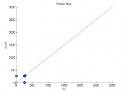
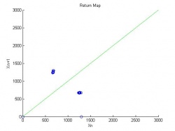
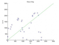
In the higher acceleration regions of the bifurcation diagrams we see that things become more chaotic. To look for more patterns in the data that may not be visible in the bifurcation diagram, return maps were generated to visualize the relationship between the time of flight for the current bounce and the one preceding it. Return maps for $\Gamma$ of 1.75, 2.25, and 3.5g are shown in Figures 9, 10 and 11.
<math>gamma=1.75</math>
<math>gamma=2.25</math>
<math>gamma=3.5</math>


Figure 9 shows a single bounce mode where each bounce is the same length as the previous one. This is seen by the single grouping of points along the one to one line. Figure 10, shows a two bounce mode where two distinct bounces are seen on either side of the one to one line. Both of these return diagrams can be inferred from looking at the bifurcation diagram. Figure 11 shows the return diagram for a more interesting region. In the region of $\Gamma$ = 3.5 the bifurcation diagram looks very chaotic; however, the return map shows clear patterns in the data. A bimodal curve is seen in the bifurcation diagram indication complex behaving is being observed.
Possible Error Sources
There are few sources of error which have been identified over the course of this work. Given below is the list of these errors along with their short description:
- Low frequency vibration of the shaker plate: Slow idle vibrations in the shaker plate was observed specially at high g input accelerations. This was primarily caused by the ball impacting the plate at high velocity.
- Ball Torquing: We also observed slight twisting of the bouncing mass due to nonuniform impact with the shaker plate. There was also similar twisting of the ball during flight for high g inputs which may be also be attributed to torquing.
- In-elasticity of the bouncing ball: During our drop tests it was observed that ball doesn't immediately come to rest and has some in-elasticity associated with it. This in-elasticity was not taken into account in our theoretical models or corrected for in our experimental data.
Conclusion and Future work
In this research we have successfully studied the behavior of a completely inelastic bouncing ball on a vibrating plate subjected to a multiple sinusoidal based input forcing function. To improve the model accuracy, coulomb friction has also been incorporated in the theoretical model. Experimental impact data is acquired via a voltage based impact detection circuit. The raw voltage data is post processed in matlab to obtain the actual flight times of the bouncing ball. Bifurcation diagrams. both with the theoretical model and experimental data have been generated. The results, with friction included are a close match with the actual experimental data. Return or N+1 maps have also been generated, which show period doubling and bi-modal behavior of our dynamical system. The discrepancy between absolute TOF values maybe attributed to possible sources of error like plate idle feedback, torquing impact of the ball and elasticity of the bouncing ball. Future work may include improving the experimental setup to reduce the free vibrations in the shaker, incorporating multiple sine waves during the experiment and incorporating elasticity directly in the theoretical model.
References
<references/>