Group 2: Difference between revisions
No edit summary |
No edit summary |
||
| (66 intermediate revisions by 2 users not shown) | |||
| Line 1: | Line 1: | ||
'''Plinko dynamics''' | |||
''Group Members: Chris Cordell, Andrew Hardin, Andrew Masse'' | |||
[[Media: Plinko_Compressed.pdf| Presentation]]. '''Papers:''' [[Media: Mass_Andrew.pdf | Andrew]], [[Media: Hardin_Charles_-_Group_2_-_6268_Final_Paper.pdf | Andrew]], [[Media: Cordell_Group2_Phys6268.pdf | Chris]] | |||
Here we investigate the dynamics of a particle traveling through a periodic lattice of attractor/repellers. This problem is inspired from a pedagogical example of a chaotic system first described by Ed Lorenz, that of a free skier descending a hill with moguls (periodic bumps). | |||
[[File:Plinkoseason37.jpeg | thumb | 300px | Plinko game on The Price is Right ]] | [[File:Plinkoseason37.jpeg | thumb | 300px | Plinko game on The Price is Right ]] | ||
= | = Background = | ||
Inspired by the game [http://en.wikipedia.org/wiki/Plinko Plinko] featured on the popular American television gameshow [http://en.wikipedia.org/wiki/The_Price_Is_Right The Price is Right], | Inspired by the game [http://en.wikipedia.org/wiki/Plinko Plinko] featured on the popular American television gameshow [http://en.wikipedia.org/wiki/The_Price_Is_Right The Price is Right], the original concept was to investigate potentially chaotic structure within the Plinko system. As will be discussed briefly below, this proved to be more difficult than was initially expected, and the collision based peg system was replaced with a series of magnets to create a magnetic Plinko board. | ||
== | == Problems with Original Plinko == | ||
Traditional studies of Plinko and other pinball billiard games have analyzed the aggregate statistics of the outcomes based on the starting position [1,2]. These analyses assume that each puck-pin interaction can only result in one of two possible outcomes: left or right. These analyses also assume that the puck must always continue downward without the possibility for upward motion, and they do not analyze the trajectory or starting conditions in detail. | Traditional studies of Plinko and other pinball billiard games have analyzed the aggregate statistics of the outcomes based on the starting position [1,2]. These analyses assume that each puck-pin interaction can only result in one of two possible outcomes: left or right. These analyses also assume that the puck must always continue downward without the possibility for upward motion, and they do not analyze the trajectory or starting conditions in detail. | ||
In order to study this system, a simulation of the system has been created in two ways: using a Runge-Kutta integration method with an event detection loop to detect collisions between the puck and the pegs to solve the puck's motion due to gravity; and a simulation that calculated parabolic trajectories between pegs and root solved for the collisions. For both methods, upon the detection of a collision, the model calculates the reflection angle of the puck about the peg normal at the collision point with a user-defined coefficient of restitution. From this angle, a new initial velocity is determined and the process is iterated from that point. This procedure continues until the puck crossed the lowest row of pegs on the Plinko board. | |||
[[File:Expdiv.png | thumb | 300px | Exponential divergence of collisions ]] | |||
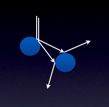
Both methods have significant problems appropriately detecting collisions. The Runge-Kutta integrator often sets the time step so high as to miss collisions due to the simple nature of the equations of motion. Fixing the time step to some small value causes collisions to be detected correctly, but this results in a longer run time as well as the build up of numerical errors in the trajectory. Running two different maximum time steps for the same initial condition results in significantly different trajectories. The parabolic simulation is mostly immune to overstepping collisions at high (>0.8) coefficients of restitution, but for values of the variable low enough to provide the dissipation necessary for the onset of chaos, even the parabolic simulation has singularity issues that led to trajectories clipping the pegs. | |||
In addition to simulation issues, a map of the initial position and velocity against the final cross-slope position reveals that there is no structure in the input space, and there are no basins of attraction within the system to the resolution to which we ran the simulation. Furthermore, no analysis of the data is able to produce a strange attractor. It is determined that this problem did not produce chaotic behavior that is qualitatively similar to the previously-studied and presumable similar pinball and billiard systems [3,4,5]. The results are, instead, distinctly random in nature and small perturbations yield extremely divergent behavior beyond even the weak chaos of ergodic motion. This is due to the exponential divergence of two similar trajectories as they evolve in the system and because there is no attractor limiting (dissipating) that divergent behavior. | |||
== Ski-Slope Dynamics == | |||
[[File:skislope.png | thumb | 250px | Mogul field on a ski-slope [6] ]] | |||
[[File:Lorenz_attractor.PNG | thumb | 250px | Progression of attractor structure descending down the ski-slope [6] ]] | |||
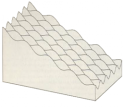
While Plinko as shown on the Price is Right is a random process, there are similar types of scenarios wherein an object descends through a regular field of obstructions that alter its trajectory as it descends. One such scenario is ski-slope dynamics [6]. In this scenario, a series of moguls are located on a slope, and a sliding object is allowed to descend under the force of gravity. As the sliding object interacts with the moguls, the trajectory is altered. | |||
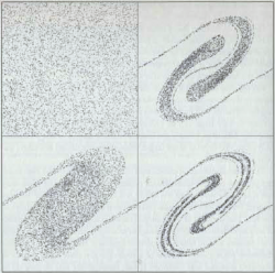
Lorenz created a simulation of this problem that shows significant chaotic behavior. Tracking cross slope velocity as a function of cross slope location for a variety of downslope positions shows the formation of an attractor, as shown in the image to the right. The progression of the attractor formation proceeds from top to bottom, then left to right as the object descends through the mogul field. Lorenz fixes downslope speed in his system, which is not totally identical to the Plinko system where the puck accelerates vertically. A fixed downslope speed can be thought of as the object reaching terminal velocity and only having the moguls redirect the trajectory, indicating that sufficient downslope is required to reach a terminal condition. The peaks of the moguls are similar in nature to the pegs of the Plinko board, in that any object approaching the peak will tend to get repelled. However, instead of a discrete collision as exists within Plinko, a ski-slope provides continuous force acting on the object. This serves to create a continuously varying trajectory which does not necessarily diverge from neighboring trajectories as was seen in Plinko. Lorenz provides a simulation which sets a framework for looking at ski-slope dynamics, but does not have experimental data to support the model. | |||
The advantage of a ski-slope problem from a simulation aspect is that the governing equations of motion are now continuously varying without the discrete collisions inherent in the Plinko system. Thus ordinary differential equation solvers will not run into the same problems encountered during the simulations of the Plinko system, where setting a maximum time step ensures collision detection at the cost of numerical errors propagating throughout the trajectory. A smoothly varying equation of motion provides a well behaved model to simulate, as well as carrying the underlying chaotic structure which Lorenz shows in the form of an attractor in position and velocity space. | |||
Combining Lorenz's observations with the original idea of investigating a Plinko board, an experiment and simulation have been developed to determine the chaotic behavior of a magnetic Plinko board. Instead of discrete collisions from a peg board, magnets will be used to continuously alter the puck trajectory as it descends through the field. Rather than using raised pegs which could still provide collisions, the magnets are embedded within the Plinko board so as to provide a smooth, unobstructed surface for the puck to slide along. This is not a perfect analog to the Lorenz simulation, as in that simulation each mogul affects the trajectory without regard to the presence of other moguls. For a magnetic Plinko board, there will be some magnetic force associated with all of the magnets in the board, not just the nearest magnet to the current point in the trajectory. Tracking of the trajectories will provide data in support of the magnetic Plinko simulation, to verify if the structures seen are physical in nature. | |||
= Methodology = | |||
To investigate the chaotic behavior of a magnetic Plinko board, both an experiment and a simulation have been set up. The experiment consists of constructing a low cost magnetic sheet which a magnetic puck can slide down. Trajectory information is collected with a camera connected to a computer with LabView software to track the motion of the puck each time it is dropped through the magnetic Plinko board. The simulation consists of MATLAB code written to model as closely as possible the physical parameters of the experimental setup. After verifying that the simulated trajectories compare qualitatively with the experimental results, an in depth investigation into the underlying attractor structure can be performed. | |||
== Experiment == | == Experiment == | ||
[[File:Skislope_exp_setup.png | thumb | 300px | Experimental Setup ]] | |||
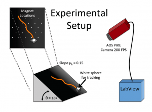
== | There are three components to the experimental setup to obtain trajectory data for the magnetic Plinko scenario. First, the puck must be constructed so that it can slide down the Plinko board. The puck is made from Teflon to reduce the friction on the puck as it slides. The Teflon houses a magnet to create the magnetic force on the puck as it slides. A ball is attached to the top of the puck for ease of tracking with the camera system. | ||
[[File: | Next, the puck needs a magnetic Plinko board to slide down. Rare earth magnets have been inserted into a Plexiglas sheet that was predrilled to have a series of holes in a triangular formation with approximately 3 cm spacing. In this configuration, the magnets attract the puck, meaning that the magnet sheet represents the basins between moguls of the ski-slope dynamics problem. This sheet was found to create too strong of a magnet field by itself, as the puck would tend to attract to the magnets or flip over and fall off the board as it passed. To reduce the strength of the magnetic forces while still providing a sufficient force to noticeably alter the trajectories, a thin sheet of plastic was added to the top of the Plexiglas. This served to increase the distance between the Plinko board magnets and the puck magnet, which reduced the overall force. A total of 28 magnets distributed over 5 rows create the final magnet sheet. The plastic is black so that the ball on top of the puck is easily distinguishable. | ||
Lastly, a camera system is required to capture the trajectories of the puck as it descends through the magnet sheet. An Allied Vision Technologies PIKE camera was connected to a computer and LabView was used for real time tracking and data collection of each run. LabView tracks the white ball on top of the puck at 200 frames per second, which shows up clearly against the totally black backdrop of the Plinko board. Trajectories are recorded in dimensions of pixels from the camera system. | |||
Experiments would be conducted by starting the puck in one of four regions near the cross-slope center line. Two regions would be on the center line at slightly varying heights. The other two regions would be slightly offset from the center line (to the right) and at equal heights to the previous two regions. The puck would be placed into each of the four regions and released without imparting initial velocity or spin. Preliminary testing in simulation showed some interesting dynamics in the repulsive case; however, the initial trials showed that the puck was prone to flipping in the repulsive configuration. The experiment and simulation were reconfigured to test the attracting condition which proved to be more stable. This should still be a consistent model with the ski-slope dynamics, as the basins between moguls are effectively attracting the trajectories. 100 runs were performed from each initial drop region, for a total of 400 runs. The time and position history data for each run was saved for later analysis. | |||
== Simulation == | |||
To simulate the magnetic Plinko board, a MATLAB code has been written to integrate the equations of motion for the puck, taking into account accelerations due to gravity, friction, and the magnets as shown below. The gravitational acceleration depends on the tilt angle of the board. The acceleration due to friction depends on the tilt angle of the board and the kinetic friction coefficient. The direction of this force is opposite that of the velocity vector, but not dependent on the puck velocity. The acceleration from the magnets is modeled as a 1/r^2 function, which should be valid for small magnets spaced far apart. This force is determined for each magnet and summed together to get the net magnetic force. A negative value of the coefficient represents an attracting magnet while a positive coefficient represents a repelling magnet. Each of these forces is written in the frame of the magnetic sheet, where X is cross slope position and Y is downslope position. The origin is set to be the lower left magnet on the magnet sheet. | |||
:<math>\vec{a}_{g} = [0,-g\cdot\sin\theta]</math> | |||
:<math>\vec{a}_{f} = -\mu\cdot g\cdot \cos\theta \left [ \frac{V_x}{V},\frac{V_y}{V} \right ]</math> | |||
:<math>\vec{a}_{m} = \sum_{i=1}^{N_{magnets}}\left (\frac{k}{{R_{i}}^2}\right)\cdot \hat{R_i}</math> | |||
[[File:R2_finalx.png | thumb | 300px | Mapping of final cross-slope position to initial-cross slope position and magnetic force coefficient ]] | |||
To have the simulation match as closely as possible with the experiment, the parameters in the equations above need to be determined. The angle of the board is measured from the experimental setup. The coefficient of kinetic friction is estimated as the tangent of the angle where puck motion could be sustained. The magnet depth is measured from the construction of the board. To determine the correct coefficient for the magnetic force equation, a trade study is performed, varying initial cross-slope position and magnetic force coefficient until the trajectories qualitatively resemble those seen in the experiment. As is shown in the image to the right, the magnetic force eventually saturates the system, and the trajectories converge to the same paths. Thus the value shown in the table was chosen, as it represents trajectories which agree well with the experiment. | |||
{|style="background:white; border:1px solid dimgray;color:black" border="1" align="center" valign="bottom" cellpadding=5px cellspacing=0px | |||
|+style="background:white; color:black"|''Simulation parameters'' | |||
|-align="left" valign="top" | |||
!Parameter | |||
!Value | |||
|-align="left" valign="top" | |||
|Tilt Angle | |||
< | |18<math>^{\circ}</math> | ||
|-align="left" valign="top" | |||
|Gravity | |||
|9.81 <math>\frac{m}{s^2}</math> | |||
== | |-align="left" valign="top" | ||
|Kinetic Friction | |||
|0.15 | |||
|-align="left" valign="top" | |||
|Magnet Depth | |||
|0.5 cm | |||
== | |-align="left" valign="top" | ||
|Magnetic Force Coefficient | |||
| -0.005 | |||
== References | |} | ||
= Results and Analysis = | |||
The experimental data has been reduced to show the full trajectory of each run as well as plots of the cross-slope velocity as a function of cross-slope position as the magnet passes each row of magnets. Video has been created of some runs to demonstrate the experimental method. The simulation has been run to generate basins of attraction for initial conditions covering half of the horizontal spread of the Plinko board. Additionally, a sequence of data points have been run at a constant drop height and varying initial cross-slope location to generate attractor structure similar to that seen in the Lorenz simulations. | |||
== Trajectory Analysis == | |||
The two videos shown below are taken from the experimental data. The first video shows a sequence of 5 runs to demonstrate the experimental process. A wand is used to hold the puck stationary, then lifted to release the puck into the magnetic sheet. This video also shows the sensitive dependence on initial conditions, as each puck drop is fairly close to the others, yet the trajectories vary. Some of the drops tend to want to converge to the same path, a result most likely due to symmetry in the magnetic forces causing the puck to follow vertical or diagonal paths. There is also a repeatability to the runs, as the first and last run are almost identical. The run with a hitch in its path demonstrates a potential source of error in the experimental data, as the puck needs to be periodically wiped down because it acquires dust which causes it to have a much higher friction force. Thus it will slow too much, and either stop on the board or be strongly attracted by the nearest magnet. | |||
The second video and the image below show the trajectories for each run plotted with each other. The trajectories tend to follow the paths of least resistance, which means either a vertical drop or a diagonal row of magnets. If the puck passes near to a magnet, then its trajectory will be deflected such that it follows a diagonal. Since the initial conditions are clustered in the center of the board, these trajectories have a limited number of paths which they will attempt to follow down the board. | |||
[[File:Exp_trajectories.png | thumb | 300px | All experimental trajectories ]] | |||
<videoflash>Tmf18EciFQs</videoflash> | |||
[[File:R2_trajectories.png | thumb | 300px | Simulation trajectories ]] | |||
<videoflash>3o23-CVlYyA</videoflash> | |||
The image above shows a sampling of the trajectories from the numerical simulation. These trajectories are generated with the parameters shown in the table above. These trajectories show similar paths to that seen in the experimental results. The puck tends to follow either a vertical path passing over magnets aligned in that direction, or gets perturbed onto a diagonally aligned row of magnets. Whichever path is taken depends on the proximity of the puck to the magnets as it descends, as it must pass near to a magnet to have sufficient force to perturb the trajectory onto a diagonal. | |||
== Basins of Attraction == | |||
[[File:Row5.png | thumb | 250px | Mapping of final cross-slope position to initial conditions ]] | |||
The image to the right shows a mapping of final cross-slope position for a range of initial conditions. Since the mapping should be symmetric about the center of the Plinko board, only one half of the initial condition space is shown. Initial cross-slope varies from 0.5 to 7.5 cm and initial height varies from 12 to 16 cm. As the initial drop height increases, the puck has a greater speed when passing the first row of magnets. Thus, the trajectories are less affected by the magnets since the puck moves through the magnetic sheet quicker. For drop heights just above the magnet sheet, the puck has not built up enough speed to shoot through the system relatively unperturbed, and more interesting dynamics exist. In particular the regions where a puck passes just to left or right of a magnet show a tendency to attract to the same final state. This is consistent with the results seen in the trajectories themselves, as the tendency is for trajectories to converge to similar paths through the magnet sheet. Interestingly, there are regions that demonstrate sensitive dependence on the initial conditions, where small variations result in much different final states. A more refined investigation in these regions did not reveal a fractal structure. There is no repeating of this effect at smaller dimensions, which is not unexpected since these effects are most likely due to the magnet trajectory being perturbed by a magnet lower down the slope instead of a magnet in the top row. | |||
== Attractor Structure == | |||
[[File:Combined_row2speed.png | thumb | 150px | Velocity versus cross-slope position passing row 2 ]] | |||
=== Total Speed === | |||
The phase space of the system was reduced in two ways in order to reconstruct the attractor. In the first method, a set of initial x conditions was selected that spanned a portion of the cross-slope. The speed magnitude of the puck was then observed as it passed each row of magnets and the initial cross-slope x position was plotted against the speed magnitude at each row of magnets, shown for row 2 in the image at the right. | |||
This shows an interesting albeit somewhat expected result: the experiment and the simulation show similar qualitative behavior in the region highlighted on the figure. This means that even in a transient region of the system (near the start of the puck trajectory) the simulation model matches the physical system quite well. It should be noted that much of the difference between the two plots is in the density (or lack thereof) of data points in the physical experiment. Additional data would help to resolve the attractor. | |||
While an interesting result, the comparison begins to break down the further the puck traverses the slope. This is because of the small number of data points in the experiment and the fact that the attractor tends to scatter these points along the map due to their slight differences in initial conditions. What is of interest is that there is a definite order to the evolution of the puck's motion from an ordered, square field of initial conditions to an equally-ordered, folded and contracted phase space after only a short period of time. | |||
[[File:Combined_row1xvx.png | thumb | 150px | Cross-slope velocity versus cross-slope position passing row 1 ]] | |||
[[File:Combined_row3xvx.png | thumb | 150px | Cross-slope velocity versus cross-slope position passing row 3 ]] | |||
=== Cross-slope Speed === | |||
Equally interesting and better suited for comparison is the second reduction method. In this method, a line of co-altitude initial points (same y value) was selected that spanned a portion of the cross-slope with various initial x positions included in the set. The cross-slope velocity (magnitude and direction), u, of the puck was then observed as it passed each row of magnets and the initial cross-slope x position was plotted against the velocity at each row of magnets. This is shown for both row 1 and row 3 in the images to the right. | |||
This result is far more interesting for several reasons. First, the results of the simulation and experiment remain comparable. The data at Row 1 bears this out clearly; the data at Row 3 , while less immediately clear, can be seen to have a similar qualitative behavior to that predicted by the simulation; there is a difference in the sign of the mean slope of the graphs, owing to the right-biased offset in the experimental data. This can be visually rectified by focusing on the region of the simulated results just left of the vertical center line. Since the initial condition space for the experiment is a much reduced version of that used in the simulation, the data points for the experiment are most likely a small subset of the attractor structure consistent with that seen near the center of the structure in the simulation data. In particular, there is a slight upslope in the simulation data for a small region around the center, which appears to have a similar number of peaks to that seen in the experimental dataset. Performing a similar comparison at row 4 or row 5 is not possible due to the limited number of experimental data points. | |||
The second reason for the increased interest in this attractor construction method is due to the more obvious folding and contraction of the phase space. It is quite clear at this point that there is a definite order and symmetry to the time evolution of the puck due entirely to the starting position. What is more, it can been shown through visual inspection that there are motions that are essentially disallowed by the physics of the system. A puck starting to the right of its nearest peg will go left, and a puck starting to the left of its nearest peg will go right (exactly as expected for the attracting case). However, as the system evolves, there are breaks in this symmetry. Looking at Row 3, there are portions of the phase space where the puck encounters a "decision" in that very slight differences in the starting position will cause it to either maintain its diagonal trajectory, reverse directions, or begin a near-vertical descent (the puck will always have an odd number of possibilities stemming from the choice of going high or low on the current trajectory, high or low on the reverse trajectory, or vertical). At each row of magnets, the number of possibilities increases with 1+2(n-1) where n is the current row number. | |||
When looking at the simulation attractor structure as the puck passes row 3, it appears to be qualitatively similar to that seen in the Lorenz simulation. There is a certain folding structure visible as each row of magnets is passed, which evolves in a similar manner to the Lorenz image shown previously. This is not an exact comparison since the underlying physics being modeled are different between the two simulations, but the similarities show that the problems represent similar ski-slope dynamical systems. One key difference is that Lorenz notes that a sufficient downslope distance is required to establish the attractor structure, which is probably not being achieved in the magnetic Plinko simulation. A longer magnet sheet would provide information in this regard. | |||
===Longer-Term Behavior=== | |||
The transient region results, while interesting, only represent behavior of the system in keeping with the experiment. As the system evolves, the dynamics settle onto the final attractor and become more interesting, as shown in the image to the right. After 30 rows, a small group of similar starting positions shows that the runs remain on a remarkably similar diagonal trajectory, until they turn and begin a vertical descent. It is at this point that the attractor begins to pull these trajectories to different parts of the phase space, thus showing the sensitivity to initial conditions. | |||
[[File:Subset_long_term.png | thumb | 200px | Long-term evolution of magnetic ski slope trajectories]] | |||
In constructing the attractor that forms in the long-term evolution of the system, we hoped to see similar behavior to that of the long-term Lorenz attractor (shown above). This clear spiral was not found. Instead, the phase space is just showing the beginnings of a collapse into ordered chaos. A longer runtime would have, yet again, provided more insight. There are, however, a few notable features of the attractor. The diagonal and vertical attracting trajectories can be easily seen beginning to form globally. This clearly ordered system that is beginning to form demonstrates the oscillatory nature of nearby trajectory groups to repeatedly go between vertical and diagonal lines (the paths of least resistance in the Lorenz ski slope and the paths of highest magnetic attraction in the magnetic ski slope) and eventually diverging. | |||
[[File:Long_term_row_30.png | thumb | 300px | Long-term evolution of the attractor shows a contraction and the formation of clear structures]] | |||
The dissimilarities between the Lorenz system and the magnetic system are likely due to three main contributions. The first is obvious: the Lorenz system is a passive force system whereas our magnetic system produces active attracting force on the puck at all times and from all pegs. That said, the forces of pegs not near the puck are nearly zero (thus why the finite span of magnets is an acceptable configuration and also likely the cause of the 1:1 trajectory behavior) and aid in keeping the overall nature of our system similar to the Lorenz system. The second significant difference is the set of simplifying assumptions. In the Lorenz study, the downhill speed of the puck is fixed; in this system, it is not fixed and depends on gravity and magnetic attraction which speeds and slows the puck. The Lorenz system is therefore semi-conservative as energy lost or gained from the slope is matched by the puck speeding up or slowing. The final difference is that the Lorenz system was integrated over a much longer slope, allowing the system to fully evolve. Due to computational and schedule limitations, this was not possible for our system. | |||
= Conclusions = | |||
A magnetic Plinko board exhibits characteristics which are consistent with results seen for a ski-slope dynamics problem. Clear basins of attraction form for a magnetic puck dropping through a sheet of magnets, particularly when the puck initially passes close to one of the magnets. Mapping cross-slope velocity against cross-slope location as the puck travels down the Plinko board shows the formation of a folded structure similar to that seen in Lorenz's ski-slope dynamics simulation. Experimental results and simulation results of the magnetic Plinko board are in qualitative agreement under the assumptions made for the values of modeling parameters in the simulation. Inconsistencies arise due to physical errors and uncertainties in the Plinko board, location of magnets, and determination of relevant parameters that limits direct quanitative comparison. Limitations in the experimental setup due to the puck falling off the side of the Plinko board prevented acquisition of data for initial conditions located far off center, which also limited the ability to validate the simulation results with the experiment. What qualitative data was taken shows an attractor structure that is similar in shape between the simulation and experiment, indicating that the simulation is a good model for the puck traveling through the magnet sheet. | |||
To further investigate the chaotic structure of magnetic Plinko, more experimental data points would need to be taken. Determining a method to allow for a wider range of initial conditions would allow for a more thorough construction of the attractor as the puck passes each row of magnets. Within the simulation, running a finer resolution sweep of initial conditions would better fill in the structure of the attractor for magnet rows further down the board. Improving the models for the magnetic force would also potentially affect the attractor shape. A series of rare earth magnets will create a complicated magnetic field that is not being modeled in the current simulation. Some of these underlying magnetic field interactions may better explain the tendency of the puck to travel along certain paths as it descends through the magnet sheet. A longer magnetic Plinko board allows for further tracking of the formation of the attractor, which may show better agreement with the Lorenz simulation that tracked trajectories for a large downslope distance. | |||
= References = | |||
[1] http://phet.colorado.edu/en/simulation/plinko-probability. Plinko Probability. University of Colorado Active Simulations. | [1] http://phet.colorado.edu/en/simulation/plinko-probability. Plinko Probability. University of Colorado Active Simulations. | ||
| Line 38: | Line 157: | ||
[5] Arroyo, A. Markarian, R. Sanders, D. P. “Bifurcations of Periodic and Chaotic Attractors in Pinball Billiards with Focusing Boundaries.” Nonlinearity. IOP Publishing. 2009. | [5] Arroyo, A. Markarian, R. Sanders, D. P. “Bifurcations of Periodic and Chaotic Attractors in Pinball Billiards with Focusing Boundaries.” Nonlinearity. IOP Publishing. 2009. | ||
[6] Lorenz, E. "The Essence of Chaos." The Jessie and John Danz Lectures. UCL Press, 1995. | |||
Latest revision as of 09:59, 12 January 2012
Plinko dynamics
Group Members: Chris Cordell, Andrew Hardin, Andrew Masse
Presentation. Papers: Andrew, Andrew, Chris
Here we investigate the dynamics of a particle traveling through a periodic lattice of attractor/repellers. This problem is inspired from a pedagogical example of a chaotic system first described by Ed Lorenz, that of a free skier descending a hill with moguls (periodic bumps).

Background
Inspired by the game Plinko featured on the popular American television gameshow The Price is Right, the original concept was to investigate potentially chaotic structure within the Plinko system. As will be discussed briefly below, this proved to be more difficult than was initially expected, and the collision based peg system was replaced with a series of magnets to create a magnetic Plinko board.
Problems with Original Plinko
Traditional studies of Plinko and other pinball billiard games have analyzed the aggregate statistics of the outcomes based on the starting position [1,2]. These analyses assume that each puck-pin interaction can only result in one of two possible outcomes: left or right. These analyses also assume that the puck must always continue downward without the possibility for upward motion, and they do not analyze the trajectory or starting conditions in detail.
In order to study this system, a simulation of the system has been created in two ways: using a Runge-Kutta integration method with an event detection loop to detect collisions between the puck and the pegs to solve the puck's motion due to gravity; and a simulation that calculated parabolic trajectories between pegs and root solved for the collisions. For both methods, upon the detection of a collision, the model calculates the reflection angle of the puck about the peg normal at the collision point with a user-defined coefficient of restitution. From this angle, a new initial velocity is determined and the process is iterated from that point. This procedure continues until the puck crossed the lowest row of pegs on the Plinko board.
Both methods have significant problems appropriately detecting collisions. The Runge-Kutta integrator often sets the time step so high as to miss collisions due to the simple nature of the equations of motion. Fixing the time step to some small value causes collisions to be detected correctly, but this results in a longer run time as well as the build up of numerical errors in the trajectory. Running two different maximum time steps for the same initial condition results in significantly different trajectories. The parabolic simulation is mostly immune to overstepping collisions at high (>0.8) coefficients of restitution, but for values of the variable low enough to provide the dissipation necessary for the onset of chaos, even the parabolic simulation has singularity issues that led to trajectories clipping the pegs.
In addition to simulation issues, a map of the initial position and velocity against the final cross-slope position reveals that there is no structure in the input space, and there are no basins of attraction within the system to the resolution to which we ran the simulation. Furthermore, no analysis of the data is able to produce a strange attractor. It is determined that this problem did not produce chaotic behavior that is qualitatively similar to the previously-studied and presumable similar pinball and billiard systems [3,4,5]. The results are, instead, distinctly random in nature and small perturbations yield extremely divergent behavior beyond even the weak chaos of ergodic motion. This is due to the exponential divergence of two similar trajectories as they evolve in the system and because there is no attractor limiting (dissipating) that divergent behavior.
Ski-Slope Dynamics
While Plinko as shown on the Price is Right is a random process, there are similar types of scenarios wherein an object descends through a regular field of obstructions that alter its trajectory as it descends. One such scenario is ski-slope dynamics [6]. In this scenario, a series of moguls are located on a slope, and a sliding object is allowed to descend under the force of gravity. As the sliding object interacts with the moguls, the trajectory is altered.
Lorenz created a simulation of this problem that shows significant chaotic behavior. Tracking cross slope velocity as a function of cross slope location for a variety of downslope positions shows the formation of an attractor, as shown in the image to the right. The progression of the attractor formation proceeds from top to bottom, then left to right as the object descends through the mogul field. Lorenz fixes downslope speed in his system, which is not totally identical to the Plinko system where the puck accelerates vertically. A fixed downslope speed can be thought of as the object reaching terminal velocity and only having the moguls redirect the trajectory, indicating that sufficient downslope is required to reach a terminal condition. The peaks of the moguls are similar in nature to the pegs of the Plinko board, in that any object approaching the peak will tend to get repelled. However, instead of a discrete collision as exists within Plinko, a ski-slope provides continuous force acting on the object. This serves to create a continuously varying trajectory which does not necessarily diverge from neighboring trajectories as was seen in Plinko. Lorenz provides a simulation which sets a framework for looking at ski-slope dynamics, but does not have experimental data to support the model.
The advantage of a ski-slope problem from a simulation aspect is that the governing equations of motion are now continuously varying without the discrete collisions inherent in the Plinko system. Thus ordinary differential equation solvers will not run into the same problems encountered during the simulations of the Plinko system, where setting a maximum time step ensures collision detection at the cost of numerical errors propagating throughout the trajectory. A smoothly varying equation of motion provides a well behaved model to simulate, as well as carrying the underlying chaotic structure which Lorenz shows in the form of an attractor in position and velocity space.
Combining Lorenz's observations with the original idea of investigating a Plinko board, an experiment and simulation have been developed to determine the chaotic behavior of a magnetic Plinko board. Instead of discrete collisions from a peg board, magnets will be used to continuously alter the puck trajectory as it descends through the field. Rather than using raised pegs which could still provide collisions, the magnets are embedded within the Plinko board so as to provide a smooth, unobstructed surface for the puck to slide along. This is not a perfect analog to the Lorenz simulation, as in that simulation each mogul affects the trajectory without regard to the presence of other moguls. For a magnetic Plinko board, there will be some magnetic force associated with all of the magnets in the board, not just the nearest magnet to the current point in the trajectory. Tracking of the trajectories will provide data in support of the magnetic Plinko simulation, to verify if the structures seen are physical in nature.
Methodology
To investigate the chaotic behavior of a magnetic Plinko board, both an experiment and a simulation have been set up. The experiment consists of constructing a low cost magnetic sheet which a magnetic puck can slide down. Trajectory information is collected with a camera connected to a computer with LabView software to track the motion of the puck each time it is dropped through the magnetic Plinko board. The simulation consists of MATLAB code written to model as closely as possible the physical parameters of the experimental setup. After verifying that the simulated trajectories compare qualitatively with the experimental results, an in depth investigation into the underlying attractor structure can be performed.
Experiment
There are three components to the experimental setup to obtain trajectory data for the magnetic Plinko scenario. First, the puck must be constructed so that it can slide down the Plinko board. The puck is made from Teflon to reduce the friction on the puck as it slides. The Teflon houses a magnet to create the magnetic force on the puck as it slides. A ball is attached to the top of the puck for ease of tracking with the camera system.
Next, the puck needs a magnetic Plinko board to slide down. Rare earth magnets have been inserted into a Plexiglas sheet that was predrilled to have a series of holes in a triangular formation with approximately 3 cm spacing. In this configuration, the magnets attract the puck, meaning that the magnet sheet represents the basins between moguls of the ski-slope dynamics problem. This sheet was found to create too strong of a magnet field by itself, as the puck would tend to attract to the magnets or flip over and fall off the board as it passed. To reduce the strength of the magnetic forces while still providing a sufficient force to noticeably alter the trajectories, a thin sheet of plastic was added to the top of the Plexiglas. This served to increase the distance between the Plinko board magnets and the puck magnet, which reduced the overall force. A total of 28 magnets distributed over 5 rows create the final magnet sheet. The plastic is black so that the ball on top of the puck is easily distinguishable.
Lastly, a camera system is required to capture the trajectories of the puck as it descends through the magnet sheet. An Allied Vision Technologies PIKE camera was connected to a computer and LabView was used for real time tracking and data collection of each run. LabView tracks the white ball on top of the puck at 200 frames per second, which shows up clearly against the totally black backdrop of the Plinko board. Trajectories are recorded in dimensions of pixels from the camera system.
Experiments would be conducted by starting the puck in one of four regions near the cross-slope center line. Two regions would be on the center line at slightly varying heights. The other two regions would be slightly offset from the center line (to the right) and at equal heights to the previous two regions. The puck would be placed into each of the four regions and released without imparting initial velocity or spin. Preliminary testing in simulation showed some interesting dynamics in the repulsive case; however, the initial trials showed that the puck was prone to flipping in the repulsive configuration. The experiment and simulation were reconfigured to test the attracting condition which proved to be more stable. This should still be a consistent model with the ski-slope dynamics, as the basins between moguls are effectively attracting the trajectories. 100 runs were performed from each initial drop region, for a total of 400 runs. The time and position history data for each run was saved for later analysis.
Simulation
To simulate the magnetic Plinko board, a MATLAB code has been written to integrate the equations of motion for the puck, taking into account accelerations due to gravity, friction, and the magnets as shown below. The gravitational acceleration depends on the tilt angle of the board. The acceleration due to friction depends on the tilt angle of the board and the kinetic friction coefficient. The direction of this force is opposite that of the velocity vector, but not dependent on the puck velocity. The acceleration from the magnets is modeled as a 1/r^2 function, which should be valid for small magnets spaced far apart. This force is determined for each magnet and summed together to get the net magnetic force. A negative value of the coefficient represents an attracting magnet while a positive coefficient represents a repelling magnet. Each of these forces is written in the frame of the magnetic sheet, where X is cross slope position and Y is downslope position. The origin is set to be the lower left magnet on the magnet sheet.
- <math>\vec{a}_{g} = [0,-g\cdot\sin\theta]</math>
- <math>\vec{a}_{f} = -\mu\cdot g\cdot \cos\theta \left [ \frac{V_x}{V},\frac{V_y}{V} \right ]</math>
- <math>\vec{a}_{m} = \sum_{i=1}^{N_{magnets}}\left (\frac{k}{{R_{i}}^2}\right)\cdot \hat{R_i}</math>
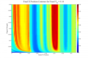
To have the simulation match as closely as possible with the experiment, the parameters in the equations above need to be determined. The angle of the board is measured from the experimental setup. The coefficient of kinetic friction is estimated as the tangent of the angle where puck motion could be sustained. The magnet depth is measured from the construction of the board. To determine the correct coefficient for the magnetic force equation, a trade study is performed, varying initial cross-slope position and magnetic force coefficient until the trajectories qualitatively resemble those seen in the experiment. As is shown in the image to the right, the magnetic force eventually saturates the system, and the trajectories converge to the same paths. Thus the value shown in the table was chosen, as it represents trajectories which agree well with the experiment.
| Parameter | Value |
|---|---|
| Tilt Angle | 18<math>^{\circ}</math> |
| Gravity | 9.81 <math>\frac{m}{s^2}</math> |
| Kinetic Friction | 0.15 |
| Magnet Depth | 0.5 cm |
| Magnetic Force Coefficient | -0.005 |
Results and Analysis
The experimental data has been reduced to show the full trajectory of each run as well as plots of the cross-slope velocity as a function of cross-slope position as the magnet passes each row of magnets. Video has been created of some runs to demonstrate the experimental method. The simulation has been run to generate basins of attraction for initial conditions covering half of the horizontal spread of the Plinko board. Additionally, a sequence of data points have been run at a constant drop height and varying initial cross-slope location to generate attractor structure similar to that seen in the Lorenz simulations.
Trajectory Analysis
The two videos shown below are taken from the experimental data. The first video shows a sequence of 5 runs to demonstrate the experimental process. A wand is used to hold the puck stationary, then lifted to release the puck into the magnetic sheet. This video also shows the sensitive dependence on initial conditions, as each puck drop is fairly close to the others, yet the trajectories vary. Some of the drops tend to want to converge to the same path, a result most likely due to symmetry in the magnetic forces causing the puck to follow vertical or diagonal paths. There is also a repeatability to the runs, as the first and last run are almost identical. The run with a hitch in its path demonstrates a potential source of error in the experimental data, as the puck needs to be periodically wiped down because it acquires dust which causes it to have a much higher friction force. Thus it will slow too much, and either stop on the board or be strongly attracted by the nearest magnet.
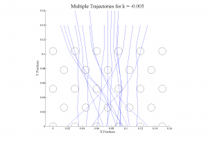
The second video and the image below show the trajectories for each run plotted with each other. The trajectories tend to follow the paths of least resistance, which means either a vertical drop or a diagonal row of magnets. If the puck passes near to a magnet, then its trajectory will be deflected such that it follows a diagonal. Since the initial conditions are clustered in the center of the board, these trajectories have a limited number of paths which they will attempt to follow down the board.

<videoflash>Tmf18EciFQs</videoflash>
<videoflash>3o23-CVlYyA</videoflash>
The image above shows a sampling of the trajectories from the numerical simulation. These trajectories are generated with the parameters shown in the table above. These trajectories show similar paths to that seen in the experimental results. The puck tends to follow either a vertical path passing over magnets aligned in that direction, or gets perturbed onto a diagonally aligned row of magnets. Whichever path is taken depends on the proximity of the puck to the magnets as it descends, as it must pass near to a magnet to have sufficient force to perturb the trajectory onto a diagonal.
Basins of Attraction
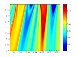
The image to the right shows a mapping of final cross-slope position for a range of initial conditions. Since the mapping should be symmetric about the center of the Plinko board, only one half of the initial condition space is shown. Initial cross-slope varies from 0.5 to 7.5 cm and initial height varies from 12 to 16 cm. As the initial drop height increases, the puck has a greater speed when passing the first row of magnets. Thus, the trajectories are less affected by the magnets since the puck moves through the magnetic sheet quicker. For drop heights just above the magnet sheet, the puck has not built up enough speed to shoot through the system relatively unperturbed, and more interesting dynamics exist. In particular the regions where a puck passes just to left or right of a magnet show a tendency to attract to the same final state. This is consistent with the results seen in the trajectories themselves, as the tendency is for trajectories to converge to similar paths through the magnet sheet. Interestingly, there are regions that demonstrate sensitive dependence on the initial conditions, where small variations result in much different final states. A more refined investigation in these regions did not reveal a fractal structure. There is no repeating of this effect at smaller dimensions, which is not unexpected since these effects are most likely due to the magnet trajectory being perturbed by a magnet lower down the slope instead of a magnet in the top row.
Attractor Structure
Total Speed
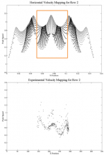
The phase space of the system was reduced in two ways in order to reconstruct the attractor. In the first method, a set of initial x conditions was selected that spanned a portion of the cross-slope. The speed magnitude of the puck was then observed as it passed each row of magnets and the initial cross-slope x position was plotted against the speed magnitude at each row of magnets, shown for row 2 in the image at the right.
This shows an interesting albeit somewhat expected result: the experiment and the simulation show similar qualitative behavior in the region highlighted on the figure. This means that even in a transient region of the system (near the start of the puck trajectory) the simulation model matches the physical system quite well. It should be noted that much of the difference between the two plots is in the density (or lack thereof) of data points in the physical experiment. Additional data would help to resolve the attractor.
While an interesting result, the comparison begins to break down the further the puck traverses the slope. This is because of the small number of data points in the experiment and the fact that the attractor tends to scatter these points along the map due to their slight differences in initial conditions. What is of interest is that there is a definite order to the evolution of the puck's motion from an ordered, square field of initial conditions to an equally-ordered, folded and contracted phase space after only a short period of time.

Cross-slope Speed
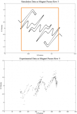
Equally interesting and better suited for comparison is the second reduction method. In this method, a line of co-altitude initial points (same y value) was selected that spanned a portion of the cross-slope with various initial x positions included in the set. The cross-slope velocity (magnitude and direction), u, of the puck was then observed as it passed each row of magnets and the initial cross-slope x position was plotted against the velocity at each row of magnets. This is shown for both row 1 and row 3 in the images to the right.
This result is far more interesting for several reasons. First, the results of the simulation and experiment remain comparable. The data at Row 1 bears this out clearly; the data at Row 3 , while less immediately clear, can be seen to have a similar qualitative behavior to that predicted by the simulation; there is a difference in the sign of the mean slope of the graphs, owing to the right-biased offset in the experimental data. This can be visually rectified by focusing on the region of the simulated results just left of the vertical center line. Since the initial condition space for the experiment is a much reduced version of that used in the simulation, the data points for the experiment are most likely a small subset of the attractor structure consistent with that seen near the center of the structure in the simulation data. In particular, there is a slight upslope in the simulation data for a small region around the center, which appears to have a similar number of peaks to that seen in the experimental dataset. Performing a similar comparison at row 4 or row 5 is not possible due to the limited number of experimental data points.
The second reason for the increased interest in this attractor construction method is due to the more obvious folding and contraction of the phase space. It is quite clear at this point that there is a definite order and symmetry to the time evolution of the puck due entirely to the starting position. What is more, it can been shown through visual inspection that there are motions that are essentially disallowed by the physics of the system. A puck starting to the right of its nearest peg will go left, and a puck starting to the left of its nearest peg will go right (exactly as expected for the attracting case). However, as the system evolves, there are breaks in this symmetry. Looking at Row 3, there are portions of the phase space where the puck encounters a "decision" in that very slight differences in the starting position will cause it to either maintain its diagonal trajectory, reverse directions, or begin a near-vertical descent (the puck will always have an odd number of possibilities stemming from the choice of going high or low on the current trajectory, high or low on the reverse trajectory, or vertical). At each row of magnets, the number of possibilities increases with 1+2(n-1) where n is the current row number.
When looking at the simulation attractor structure as the puck passes row 3, it appears to be qualitatively similar to that seen in the Lorenz simulation. There is a certain folding structure visible as each row of magnets is passed, which evolves in a similar manner to the Lorenz image shown previously. This is not an exact comparison since the underlying physics being modeled are different between the two simulations, but the similarities show that the problems represent similar ski-slope dynamical systems. One key difference is that Lorenz notes that a sufficient downslope distance is required to establish the attractor structure, which is probably not being achieved in the magnetic Plinko simulation. A longer magnet sheet would provide information in this regard.
Longer-Term Behavior
The transient region results, while interesting, only represent behavior of the system in keeping with the experiment. As the system evolves, the dynamics settle onto the final attractor and become more interesting, as shown in the image to the right. After 30 rows, a small group of similar starting positions shows that the runs remain on a remarkably similar diagonal trajectory, until they turn and begin a vertical descent. It is at this point that the attractor begins to pull these trajectories to different parts of the phase space, thus showing the sensitivity to initial conditions.
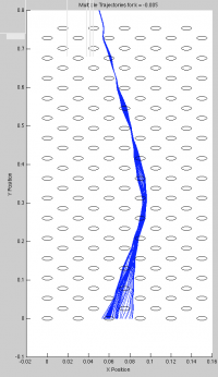
In constructing the attractor that forms in the long-term evolution of the system, we hoped to see similar behavior to that of the long-term Lorenz attractor (shown above). This clear spiral was not found. Instead, the phase space is just showing the beginnings of a collapse into ordered chaos. A longer runtime would have, yet again, provided more insight. There are, however, a few notable features of the attractor. The diagonal and vertical attracting trajectories can be easily seen beginning to form globally. This clearly ordered system that is beginning to form demonstrates the oscillatory nature of nearby trajectory groups to repeatedly go between vertical and diagonal lines (the paths of least resistance in the Lorenz ski slope and the paths of highest magnetic attraction in the magnetic ski slope) and eventually diverging.
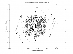
The dissimilarities between the Lorenz system and the magnetic system are likely due to three main contributions. The first is obvious: the Lorenz system is a passive force system whereas our magnetic system produces active attracting force on the puck at all times and from all pegs. That said, the forces of pegs not near the puck are nearly zero (thus why the finite span of magnets is an acceptable configuration and also likely the cause of the 1:1 trajectory behavior) and aid in keeping the overall nature of our system similar to the Lorenz system. The second significant difference is the set of simplifying assumptions. In the Lorenz study, the downhill speed of the puck is fixed; in this system, it is not fixed and depends on gravity and magnetic attraction which speeds and slows the puck. The Lorenz system is therefore semi-conservative as energy lost or gained from the slope is matched by the puck speeding up or slowing. The final difference is that the Lorenz system was integrated over a much longer slope, allowing the system to fully evolve. Due to computational and schedule limitations, this was not possible for our system.
Conclusions
A magnetic Plinko board exhibits characteristics which are consistent with results seen for a ski-slope dynamics problem. Clear basins of attraction form for a magnetic puck dropping through a sheet of magnets, particularly when the puck initially passes close to one of the magnets. Mapping cross-slope velocity against cross-slope location as the puck travels down the Plinko board shows the formation of a folded structure similar to that seen in Lorenz's ski-slope dynamics simulation. Experimental results and simulation results of the magnetic Plinko board are in qualitative agreement under the assumptions made for the values of modeling parameters in the simulation. Inconsistencies arise due to physical errors and uncertainties in the Plinko board, location of magnets, and determination of relevant parameters that limits direct quanitative comparison. Limitations in the experimental setup due to the puck falling off the side of the Plinko board prevented acquisition of data for initial conditions located far off center, which also limited the ability to validate the simulation results with the experiment. What qualitative data was taken shows an attractor structure that is similar in shape between the simulation and experiment, indicating that the simulation is a good model for the puck traveling through the magnet sheet.
To further investigate the chaotic structure of magnetic Plinko, more experimental data points would need to be taken. Determining a method to allow for a wider range of initial conditions would allow for a more thorough construction of the attractor as the puck passes each row of magnets. Within the simulation, running a finer resolution sweep of initial conditions would better fill in the structure of the attractor for magnet rows further down the board. Improving the models for the magnetic force would also potentially affect the attractor shape. A series of rare earth magnets will create a complicated magnetic field that is not being modeled in the current simulation. Some of these underlying magnetic field interactions may better explain the tendency of the puck to travel along certain paths as it descends through the magnet sheet. A longer magnetic Plinko board allows for further tracking of the formation of the attractor, which may show better agreement with the Lorenz simulation that tracked trajectories for a large downslope distance.
References
[1] http://phet.colorado.edu/en/simulation/plinko-probability. Plinko Probability. University of Colorado Active Simulations.
[2] Biesterfeld, A. “The Price (or Probability) Is Right.” University of Colorado at Boulder. Journal of Statistics Education. Volume 9, Number 3 (2001).
[3] Pring, S. R. Budd, C. J. “The Dynamics of a Simplified Pinball Machine.” University of Bath. IMA Journal of Applied Mathematics. 2011.
[4] Markarian, R. Pujals, E. J. Sambarino, M. “Pinball Billiards with Dominated Splitting.” Ergod. Th. & Dynam. Sys. Cambridge University Press. 2010.
[5] Arroyo, A. Markarian, R. Sanders, D. P. “Bifurcations of Periodic and Chaotic Attractors in Pinball Billiards with Focusing Boundaries.” Nonlinearity. IOP Publishing. 2009.
[6] Lorenz, E. "The Essence of Chaos." The Jessie and John Danz Lectures. UCL Press, 1995.